Image Compression Algorithms using Singular Value Decomposition & Fourier Transform

In this project, we will focus on the use of algorithms for dimensionality reduction. More specifically, I will apply Singular Value Decomposition (SVD) and the Fourier Transform (FT) in image compression tasks.

The goal of this project is to analyze and conclude whether SVD or FT image compression yields compressed images of higher image quality. The computational efficiency of each algorithm is also taken into account for fairer analyses.

A quick note on the rationale for comparison between these two seemingly unrelated algorithms - both the SVD and the FT are characterized by some unitary transform and expression of our data as a scaling in a different basis. Once the vector is scaled, a windowing/filtering function is introduced to identify and remove the basis vectors and frequencies which are sensitive to small changes in the data, or account for the least variance in our data. I figured it would be an interesting test to see how these two fundamentally linked algorithms perform in an image compression task.

Our dataset of images was obtained from Scikit-Learn’s skimage.data API, specifically from their “General-purpose images” collection. The two algorithms were implemented using the SVD and FFT functions in the Numpy library.

In the following sections, I will cover more details about the preliminary data analysis (with visualizations), testing methodology, result analysis with discussions and the summary of this report.

I also decided to export the original jupyter notebook in HTML format for easy reference to the code and output, so this page will read like a jupyter notebook.

This page will be segmented in the following sections:

1. Brief runthrough on the mathematical foundations of our two algorithms
2. Setting up dependencies
   1. Import packages
   2. Accessing the Image Dataset
3. Image dataset pre-analysis & visualization
   1. Writing a function to convert images to grayscale
   2. Plot Histogram of Pixel Intensity & Frequency for each image
   3. Calculate Shannon Entropy of each image
4. General testing methodology & test metrics
   1. Writing SVD compression & binary search functions
   2. Writing FT compression & binary search functions
   3. Explaining testing metrics
5. Results & analysis
   1. SVD & FFT for all images at sample compression ratio of 1.5
   2. Preliminary observations & discussion
   3. Writing a function to calculate PSNR for compressed images
   4. Plot PSNR & Computation Time for SVD & FFT on top 3 candidate images
   5. Quantitative performance analysis & discussion
6. Conclusion

1. Brief mathematical foundations for our project

In this section, I skip the mathematical derivation of each algorithm (which should be coming in a blog post soon), and touch on the primary components which will be filtered in our image compression task.

Singular Value Decomposition

The singular value decomposition of a matrix A is the factorization of A into the product of three matrices $A = U Σ V^T$ where the columns of U and V are orthonormal and the matrix Σ is diagonal with positive real entries.

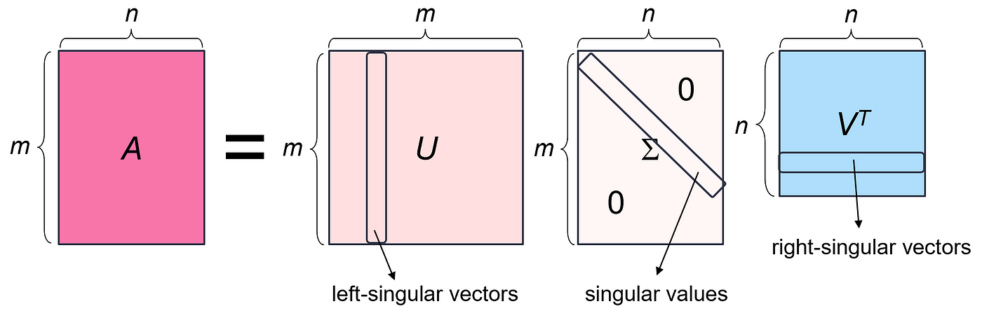
The most important factor matrix to us is Σ, which contains our singular values. This is the matrix that scales each vector before the axis system is rotated by the matrix U. We can reformulate SVD in terms of the singular values 𝝈: A = $U Σ V^T$= $𝝈_1u_1v^T_1$+ … + $𝝈_ru_rv^T_r$

Because the singular values have already been sorted descendingly in the Σ factor matrix, we know that $𝝈_1$ >= $𝝈_2$ >= (…) >= $𝝈_r$. Therefore, we can look at the first few singular values to see what the most significant direction-setting components are.

To apply this understanding to the task of image compression, we will compress an input image by removing unwanted singular values. We can approximate the matrix A by keeping only the largest K singular values and their corresponding singular vectors. Reducing K will decrease the storage requirements and the image quality, but may still provide a reasonable approximation of the original image.

Fourier Transform

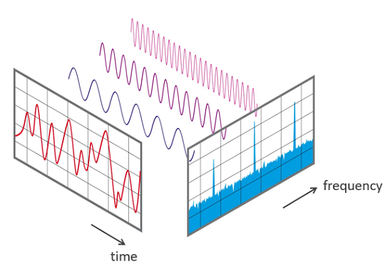
The Fourier Transform of a function or signal F(x) is a mathematical tool that decomposes (any aperiodic) F(x) into a sum of constituent sines and cosines of different frequencies.

To compute a Fourier Transform in the context of image compression, we compute the Discrete Fourier Transformation (DFT) form:

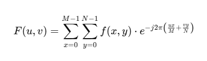
We can view the transformation in two stages, in the context of image compression:

1. A conversion from spatial (pixel) values to frequency values
2. A frequency representation where each frequency corresponds to certain image features

Geometrically, this process can be interpreted as decomposing the image into various sinusoidal patterns. Lower frequency components typically represent smooth or uniform regions in the image, while higher frequency components capture fine details and edges.

The matrix representation of the transformed image in the frequency domain is often complex-valued, with each entry containing amplitude and phase information for each frequency component. The amplitude indicates the strength of each frequency component, while the phase determines its position.

For image compression, we can leverage the Fourier Transform by retaining only the most significant frequency components and discarding less significant components. One example is to remove high-frequency components, since they usually account for finer details and edges that we may not need. This selective retention of frequencies reduces the data size but maintains essential image features. Thus, by reconstructing the image using only the dominant lower frequencies, we achieve a compressed approximation of the original image.

2. Setting up dependencies

Import packages

import matplotlib.pyplot as plt
import matplotlib
import numpy as np
import imageio
import time
import os

from skimage import data
from skimage import color

Accessing the image dataset

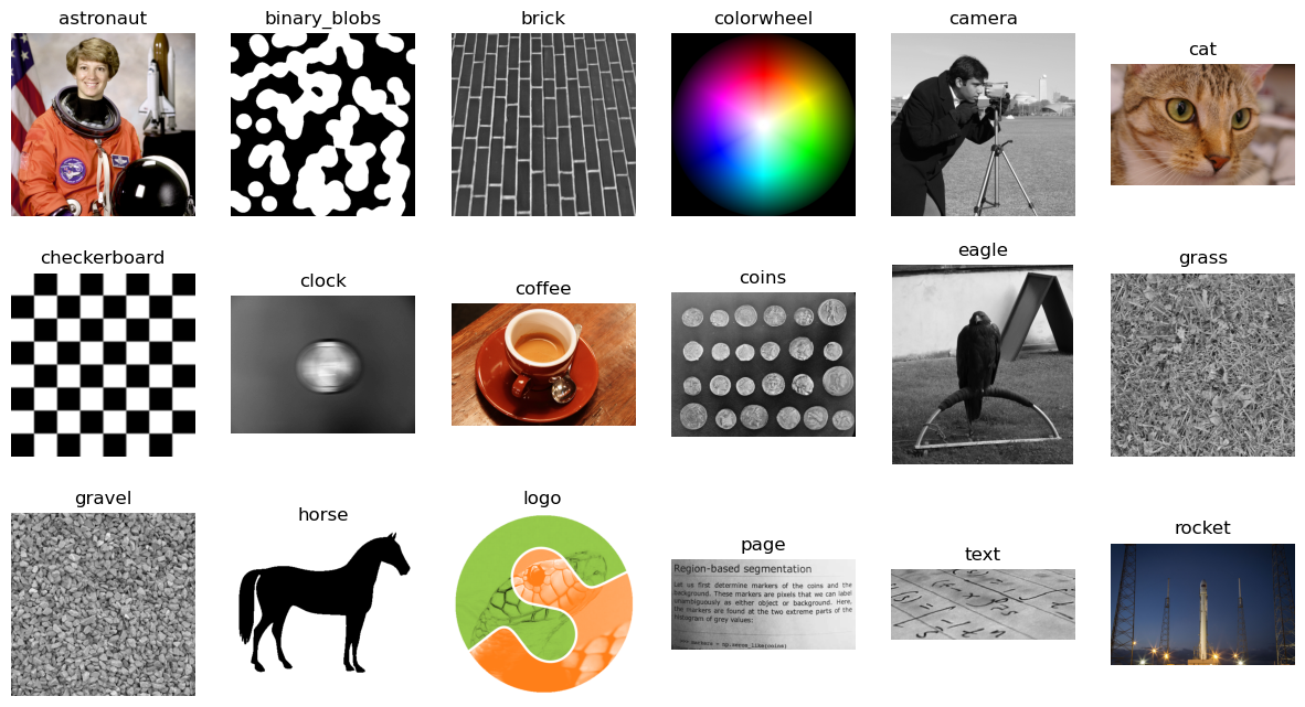
Our image dataset is accessed through the skimage API. Because I chose to work with skimage’s “General Images” collection, we have to type in the names of the 18 images that belong to that collection, under the “images” tuple below. Then, we access attributes that belong to each image, such as the image and name, using the getattr() function. Finally, we plot the images to see what they look like.

images = (
    'astronaut',
    'binary_blobs',
    'brick',
    'colorwheel',
    'camera',
    'cat',
    'checkerboard',
    'clock',
    'coffee',
    'coins',
    'eagle',
    'grass',
    'gravel',
    'horse',
    'logo',
    'page',
    'text',
    'rocket',
)

# Create subplot space for image dataset
fig, axes = plt.subplots(3, 6, figsize=(15,8))

# Loop over images and axes together
for name, axes in zip(images, axes.flat):
    caller = getattr(data, name)
    image = caller()
    axes.imshow(image, cmap=plt.cm.gray if image.ndim == 2 else None)
    axes.set_title(name)
    axes.axis('off')  # Hide axis

plt.show()

3. Image dataset pre-analysis & visualization

Writing a function to convert images to grayscale

Some of the images in the dataset come in grayscale, RGB and even RGBA. In order to have consistency and simplicity when working with these images, I chose to convert all of them to grayscale, in uint8 format. To handle that conversion, I wrote the following function, image_to_grayscale, which handles the varying dimensionality of each grayscale, RGB, and RGBA image.

def image_to_greyscale(image_array):

    # Handle color images
    if image_array.ndim == 3:
        if image_array.shape[2] == 3:  # Convert RGB to grayscale
            image_grey = color.rgb2gray(image_array)  
            image_grey = (image_grey * 255).astype(np.uint8)
            
        elif image_array.shape[2] == 4:  # Convert RGBA to grayscale by ignoring the alpha channel
            image_grey = color.rgb2gray(image_array[..., :3])  # Only take the RGB channels
            image_grey = (image_grey * 255).astype(np.uint8)
            
        else:
            raise ValueError("Unsupported number of channels. Must be 3 (RGB) or 4 (RGBA).")

    # Handle binary images
    elif image_array.ndim == 2 and image_array.dtype == bool:
        image_grey = image_array.astype(np.uint8) * 255  # Convert True to 255 and False to 0

    # Handle grayscale images
    elif image_array.ndim == 2 and image_array.dtype == np.uint8:
        image_grey = image_array  # Already grayscale

    else:
        raise ValueError("Unsupported image format or dtype")

    return image_grey

Plotting a histogram of Pixel Intensity & Frequency for each image

Here, we plot the frequency of the pixel intensity within each image matrix. These histogram plots will allow us to visually understand the general complexity of each grayscale image. It will also serve as a preparatory step before we quantify the complexity of each image usingShannon Entropy.

In the context of our small image dataset, these steps aren’t critical, but may yield some interesting observations nonetheless.

# Create a figure with a 6x3 grid of subplots for histograms
fig, axes = plt.subplots(6, 3, figsize=(15, 20))
fig.tight_layout(pad=3.0)

# Loop over images and axes to plot histograms
for name, axes in zip(images, axes.flat):
    image_array = getattr(data, name)()
    image_grey = image_to_greyscale(image_array)

    # Calculate the histogram
    hist, bin_edges = np.histogram(image_grey, bins=256, range=(0, 255))

    # Plot the histogram
    axes.plot(bin_edges[:-1], hist, color="black")  # bin_edges[:-1] aligns with hist
    axes.set_title(name)
    axes.set_xlabel("Pixel Intensity")
    axes.set_ylabel("Frequency")

plt.show()

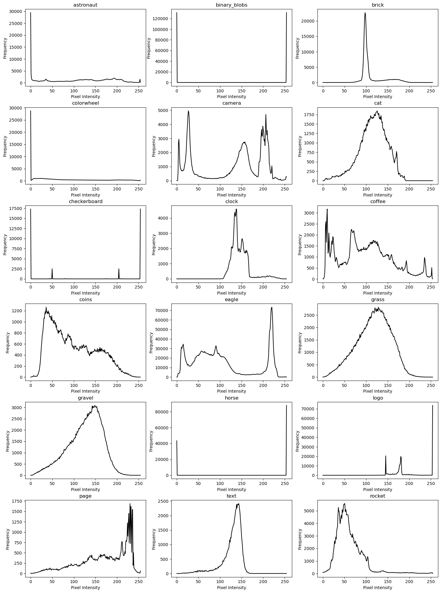
We can observe some expected correspondence between the Pixel intensity graphs and the original images.

On a very general basis, images containing photographs of natural subjects, such as “camera” and “cat” have busier plots, while “brick”, “binary_blobs” and “horse” have simpler plots.

Images like the “checkerboard” have a starkly symmetrical plot, which corresponds with their repeating patterns.

Amother interesting observation is that strongly “texture-focused” images like ‘grass’ and ‘gravel’ have pixel intensity plots which roughly resemble a gaussian-like probability distribution.

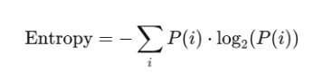
Calculate Shannon Entropy for each image

Now, we quantify the complexity of each grayscale image by calculating the shannon entropy from pixel intensity values. Again, I don’t think this is a particularly crucial step, but it does provide some quantitative pre-analysis of our dataset, and may yield some interesting insights.

Here’s the mathematical formula we’re using for Shannon Entropy, with log base 2 to measure entropy in bits.

def calculate_entropy(image_grey, name):

    # Calculate the histogram
    hist, bin_edges = np.histogram(image_grey, bins=256, range=(0, 255))
    
    # Normalize the histogram to get probabilities
    hist_normalized = hist / hist.sum()
    
    # Remove zero probabilities to avoid log2(0)
    hist_nonzero = hist_normalized[hist_normalized > 0]
    
    # Compute entropy
    entropy = -np.sum(hist_nonzero * np.log2(hist_nonzero))
    return entropy


# Store the results in a list of tuples (name, entropy)
results = []

for name in images:
    image_array = getattr(data, name)()
    image_grey = image_to_greyscale(image_array)
    entropy_value = calculate_entropy(image_grey, name)
    results.append((name, entropy_value))

# Sort results by entropy in descending order
sorted_results = sorted(results, key=lambda x: x[1], reverse=True)

# Print sorted results
for name, entropy in sorted_results:
    print(f"{name}: {entropy}")

coffee: 7.661570369288201
coins: 7.524412237976031
astronaut: 7.444158328824859
page: 7.443679900610648
eagle: 7.4014811794262005
grass: 7.288338951598444
gravel: 7.253146960346441
camera: 7.231695011055704
cat: 7.004601864511788
colorwheel: 6.911928827078324
rocket: 6.669767402285822
text: 6.13372198445881
clock: 6.0355022558653415
brick: 5.455265334504446
logo: 4.548489581745522
checkerboard: 1.6317676229974185
binary_blobs: 1.0
horse: 0.9158271515170937

4. General testing methodology & test metrics

For our tests, we will decompose each image with both algorithms. Then, we will conduct dimensionality reduction in the image to compress it, and regenerate the compressed image.

In order to conduct a fair test, we will compress each image by the same compression ratio for each algorithm. Compression ratio of each image is defined as follows:

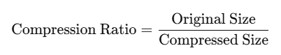
This will allow us to compare the qualities of the final output based on the “same amount of compression” done by each algorithm.

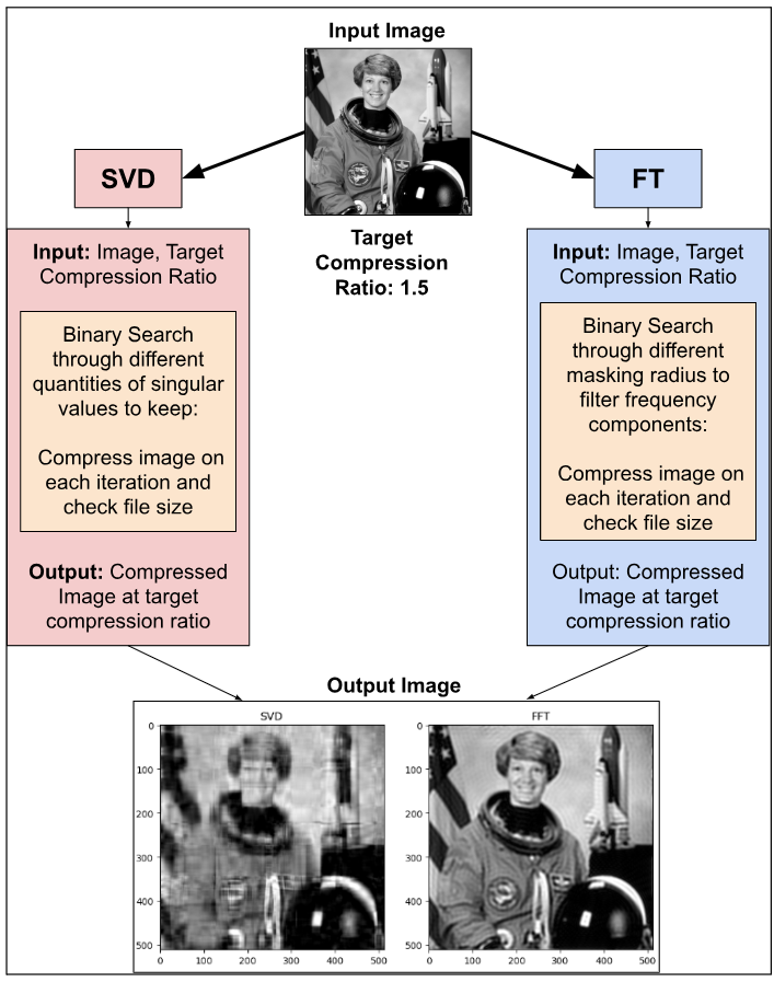
In this section, I will explain how the image decomposition and compression was done for each algorithm.

However, since nobody wants to read through huge blobs of text, here’s a diagram describing the overall workflow visually:

Implementation of the SVD Algorithm

To implement the SVD Algorithm, we used the Numpy linalg.svd function. It decomposes an input matrix into the three constituent matrices, which we can then manipulate for image compression.

After an image had been decomposed through SVD, and had its singular values removed for compression, the compressed image was reconstructed through matrix multiplication operations, then transformed into grayscale, uint8 form.

To accomplish the task of image compression within the context of this project, two functions had to be designed:

1) A compression function that removes unwanted singular values based on an input parameter that contains a predefined number of singular values to retain.

2) A function that searches for the correct number of singular values to retain, in order to enable the compressed image file size to approximate an input parameter that contains a predefined image compression ratio. To search for the optimal number of singular values to retain, a binary search was implemented.

In the code cell below, we write the two functions.

def svd_image_compress(image, num_singular_values):
    
    U, S, Vt = np.linalg.svd(image, full_matrices=False)
    U_reduced = U[:, :num_singular_values]
    S_reduced = np.diag(S[:num_singular_values])
    Vt_reduced = Vt[:num_singular_values, :]

    compressed_image_float64 = np.dot(U_reduced, np.dot(S_reduced, Vt_reduced))
    compressed_image_uint8 = np.clip(compressed_image_float64, 0, 255).astype(np.uint8)

    return compressed_image_uint8


def find_optimal_singular_values(image, target_compression_ratio, tolerance = 0.01):

    U, S, Vt = np.linalg.svd(image, full_matrices=False)

    low, high = 1, S.shape[0]
    num_singular_values = len(S)

    # Save original image to get its size
    original_image_filename = 'original_image.png'
    imageio.imwrite(original_image_filename, image)
    original_image_size = os.path.getsize(original_image_filename)

    # iteration = 0
    
    while low <= high:
        mid = (low + high) // 2
        
        # Compress image using mid value
        compressed_image_uint8 = svd_image_compress(image,mid)
        
        # Save the compressed image to calculate size
        compressed_image_filename = f'temp_compressed_image_{name}.png'
        imageio.imwrite(compressed_image_filename, compressed_image_uint8)
        compressed_image_size = os.path.getsize(compressed_image_filename)
    
        # Calculate the current compression ratio
        current_compression_ratio = round(original_image_size / compressed_image_size, 2)
        
        # Use the desired compression ratio to adjust the search bounds
        if abs(target_compression_ratio - current_compression_ratio) <= tolerance:
            num_singular_values = mid
            break
            
        elif current_compression_ratio < target_compression_ratio:
            num_singular_values = mid
            high = mid - 1
            
        else:
            num_singular_values = mid
            low = mid + 1

    return num_singular_values

Implementation of the FT Algorithm

To implement the FT Algorithm, we used the Numpy fft.fft2 function (which uses the Fast Fourier Transform (FFT) under the hood).

Firstly, we transform the input image matrix from the spatial domain into the frequency domain with the fft.fft2 function. Then we applied fft.fftshift so that the zero frequency, or lowest frequency component, was shifted to the center of the spectrum. This then enabled us to create a masking function using np.ogrid to filter out unwanted frequency components based on an input parameter which describes the radius of the open grid mask. After filtering, the spectrum plot was inverse-shifted, then the inverse FFT was applied to return our compressed image. Since the returned matrix had complex components, we also had to transform them into real pixel intensity values.

To accomplish all the above sub-tasks within the context of this project, two functions had to be designed:

1. A compression function that removes high-frequency components based on an input parameter that contains a masking radius.

2. A function that searches for the correct masking radius, in order to enable the compressed image file size to approximate an input parameter that contains a predefined image compression ratio. To search for the optimal masking radius, a binary search was also implemented.

In the code cell below, we write the two functions.

# Basic FFT Function

def apply_fft_and_mask(image,radius):

    fft_image = np.fft.fft2(image) # Transforms image to frequency domain
    fft_shifted = np.fft.fftshift(fft_image) # Shift zero frequency component to center of spectrum
    
    # Filter High Frequency Components
    rows, cols = image.shape
    center_row, center_col = rows//2, cols//2 # Center of image
    
    mask = np.zeros((rows, cols), dtype=np.uint8) # This mask will eventually contain 1's in the area corresponding to low freqs, 0's elsewhere.
    y, x = np.ogrid[-center_row:rows-center_row, -center_col:cols-center_col] # This centers your y,x variables with "center_row, center_col"
    mask_area = x**2 + y**2 <= radius**2 
    mask[mask_area] = 1 # Set masking condition for filtering
    
    fft_shifted_filtered = fft_shifted * mask
    
    # Reconstruct compressed image with Inverse FFT
    
    fft_compressed_unshifted = np.fft.ifftshift(fft_shifted_filtered)
    compressed_image = np.fft.ifft2(fft_compressed_unshifted)
    compressed_image_real = np.abs(compressed_image) # IFFT of complex frequency domain returns complex output. We want real pixel intensity values.
    compressed_image_clipped = np.clip(compressed_image_real, 0, 255)
    compressed_image_uint8 = compressed_image_clipped.astype(np.uint8)
    
    return compressed_image_uint8


# Binary Search for correct filtering radius based off defined compression ratio

def find_optimal_radius(image, target_compression_ratio, tolerance=0.02):

    rows, cols = image.shape

    max_radius = int(np.sqrt((rows/2)**2 + (cols/2)**2))

    low, high = 0, max_radius

    original_image_filename = 'original_image.png'
    imageio.imwrite(original_image_filename, image_grey)
    original_image_size = os.path.getsize(original_image_filename)

    optimal_radius = max_radius # Default value
   
    while low <= high:

        mid = (low + high)//2

        compressed_image = apply_fft_and_mask(image, mid)
        compressed_image_filename = 'compressed_image_temp.png'
        imageio.imwrite(compressed_image_filename, compressed_image)
        compressed_image_size = os.path.getsize(compressed_image_filename)

        compression_ratio = round(original_image_size / compressed_image_size, 2)
        
        if abs(compression_ratio - target_compression_ratio) <= tolerance:
            optimal_radius = mid
            break
            
        elif compression_ratio < target_compression_ratio:
            optimal_radius = mid
            high = mid -1
            
        else:
            optimal_radius = mid
            low = mid + 1
            
    return optimal_radius

Technical notes on the Compression & Search functionality

1. To save the original and compressed images into image files for file size comparison, we used the .PNG file format, because it does not introduce any lossy compression in the process.

2. There was a tolerance given to each algorithm’s compression ratio during the binary search, because the level of compression precision afforded by each algorithm is inherently different. For example, we do compression in SVD by removing singular values one-by-one. Therefore, the precision of our compression is limited by the magnitude of the singular value, and the number of singular values.

Explaining the testing metrics

In order to assess the performance of the two image compression algorithms in Section 5, we need to ensure that we are collecting data that fits our performance metrics.

We chose to use the following three quantitative metrics for our assessments:

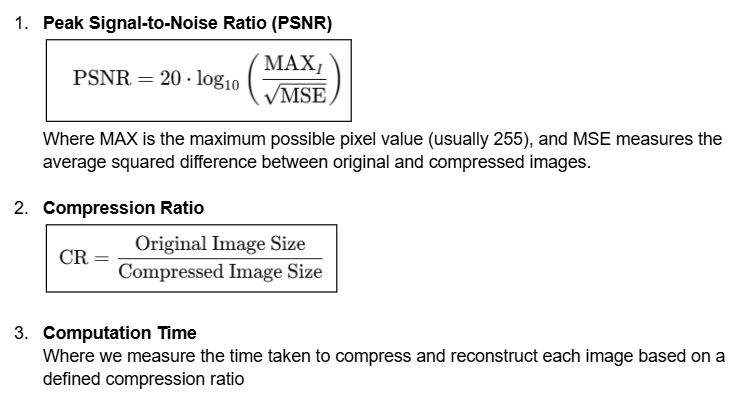
While there are other quantitative metrics to evaluate image quality loss, such as Structural Similarity Index (SSIM), and simple ones like Mean Squared Error (MSE), we decided that PSNR is a good general metric for loss of image quality, and it is widely used in image compression tools as a primary metric as well. For simplicity’s sake, we will use PSNR.

In addition, there will be qualitative metrics like our own human-perceived quality measure of image quality.

5. Results & Analysis

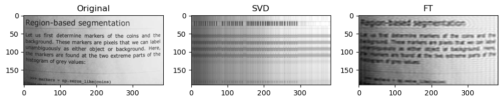
In this section, we will firstly visualize the results of image compression for a sample compression ratio of 1.5.

Then, we will discuss some interesting observations, and discuss their potential root causes.

Finally, we will use our quantitative metrics to analyze our images and discuss some of the quantitative results.

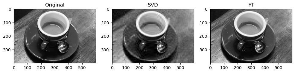
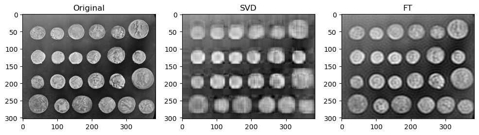
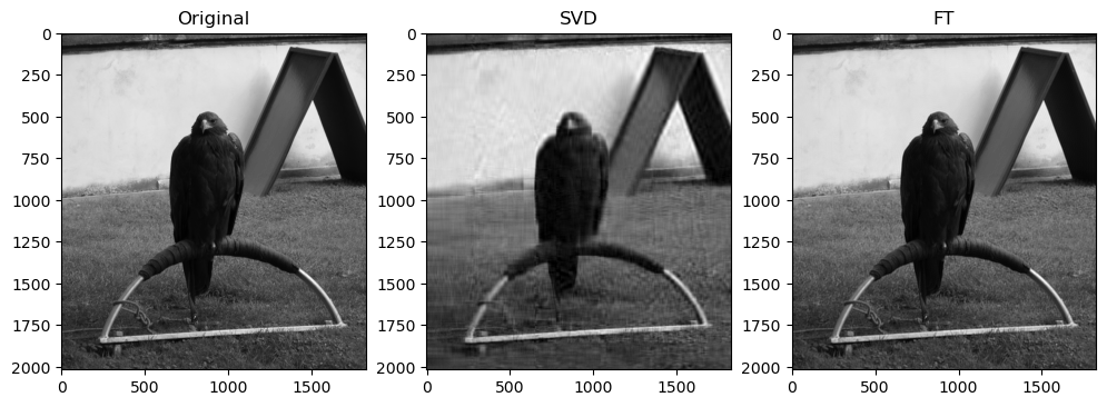
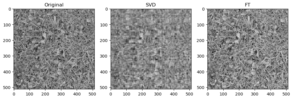
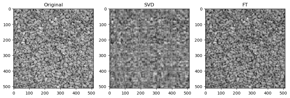
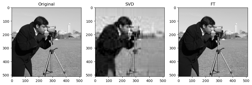
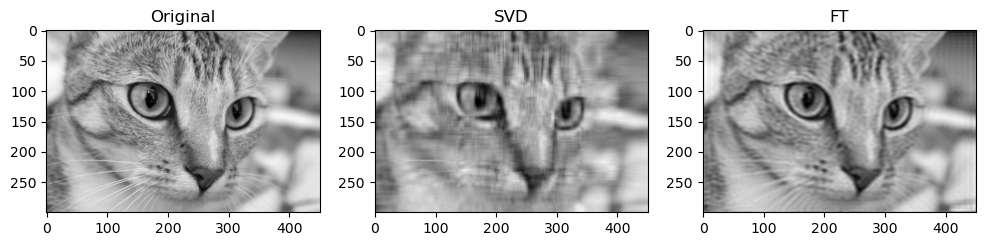
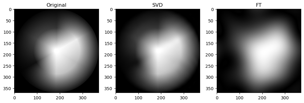
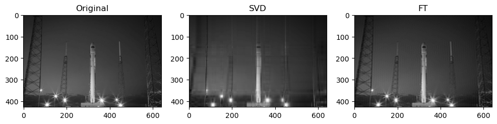
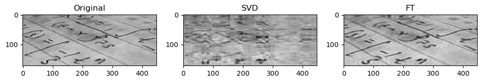
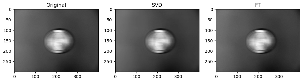
SVD & FT for all images at sample compression ratio of 1.5

Here, we apply the above SVD and FT operations on all images in our dataset, for a sample compression ratio of 1.5. We also captured details about compressed image size (original_image_size, compressed_image_size_svd, compressed_image_size_fft) and also computation time (elapsed_time_svd, elapsed_time_fft) in preparation for our later sections involving quantitative analysis.

sorted_images = (
    'coffee',
    'coins',
    'astronaut',
    'page',
    'eagle',
    'grass',
    'gravel',
    'camera',
    'cat',
    'colorwheel',
    'rocket',
    'text',
    'clock',
    'brick',
    'logo',
    'checkerboard',
    'binary_blobs',
    'horse')


for name in sorted_images:

    start_time_svd = time.time()
    
    image_array = getattr(data, name)()
    image_grey = image_to_greyscale(image_array)


    target_compression_ratio = 1.5
    
    
    num_singular_values = find_optimal_singular_values(image_grey, target_compression_ratio)
    compressed_image_svd = svd_image_compress(image_grey, num_singular_values)

    elapsed_time_svd = time.time() - start_time_svd

    start_time_fft = time.time()
    
    optimal_radius = find_optimal_radius(image_grey, target_compression_ratio)
    compressed_image_fft = apply_fft_and_mask(image_grey, optimal_radius)
    
    elapsed_time_fft = time.time() - start_time_fft
    
    original_image_filename = f'original_image_{name}.png'
    imageio.imwrite(original_image_filename, image_grey)
    original_image_size = os.path.getsize(original_image_filename)
    
    compressed_image_filename_svd = f'compressed_image_svd_{name}.png'
    imageio.imwrite(compressed_image_filename_svd, compressed_image_svd)
    compressed_image_size_svd = os.path.getsize(compressed_image_filename_svd)
    
    compressed_image_filename_fft = f'compressed_image_fft_{name}.png'
    imageio.imwrite(compressed_image_filename_fft, compressed_image_fft)
    compressed_image_size_fft = os.path.getsize(compressed_image_filename_fft)
    
    # Plotting original and compressed images
    
    plt.figure(figsize=(12,5))
    
    plt.subplot(1, 3, 1)
    plt.imshow(image_grey, cmap='gray')
    plt.title("Original")
    
    plt.subplot(1, 3, 2)
    plt.imshow(compressed_image_svd, cmap='gray')
    plt.title("SVD")
    
    plt.subplot(1, 3, 3)
    plt.imshow(compressed_image_fft, cmap='gray')
    plt.title("FT")

Preliminary observations & discussion

In general, we can see a degradation in compression performance for both SVD and FT as the Shannon Entropy of the images decreases. For instance, at the same compression ratio of 1.5, both the SVD and FT compressed “coffee” image look closer to their original image, than compared to another case like “logo” or “horse”.

This could be because low entropy images may lack enough detail and texture to support a higher compression ratio, making the compressed image lack a lot of the (minimal) information required to look like the original image.

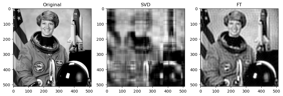
Next, when qualitatively comparing SVD and FT compression of the same image, the FT compressed image generally looks closer to the original as compared to the SVD compressed image. For instance, for “camera”:

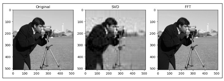
This could be because FT decomposes an image into frequency components, which is efficient at preserving periodic structures and gradual changes, which are often found in images containing natural objects. On the other hand, SVD’s non-localized basis (of singular vectors) don’t capture localized detail well, which may lead to quality loss for detailed objects.

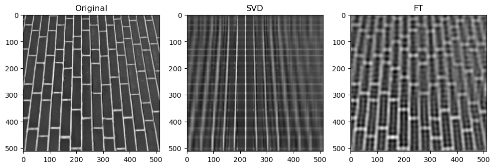
SVD compressed images that appear low quality usually have strong “orthogonal” blurriness in their compressed images. On the other hand, when a FT compressed image appears low quality, it usually has some “ringing” effect.

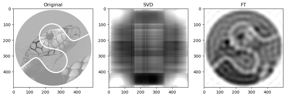
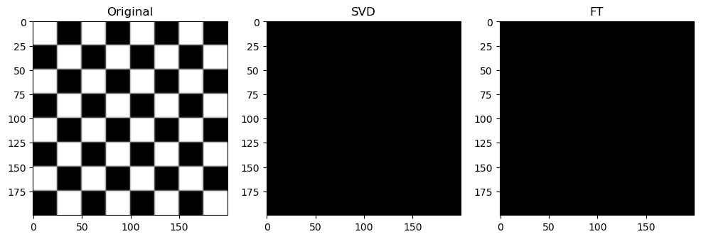
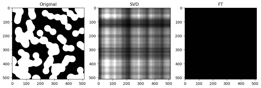
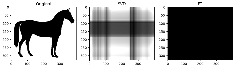
However, an interesting observation is that when the compression ratio is too high for both algorithms (usually only on images with low entropy, containing strongly simple shapes or repeating patterns), the SVD compression is able to return some “orthogonal lines” that faintly approximate the general pixel density of the original image, while the FT compression may return an empty-looking image. For example:

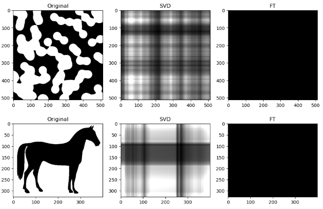
This has a very interesting consequence: the SVD-compressed images that belong in this specific situation actually have a bigger file size than the original image - meaning, after being “decomposed” into its constituent singular vectors, and reconstructing to form the above orthogonal lines, the image is actually more detailed, and takes up more storage space.

For example, the table below shows the original, SVD-compressed and FT-compressed file sizes for “binary_blob” and “horse”:

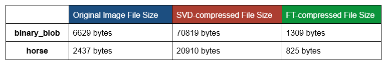
This example shows how SVD-compression might have counterproductive compression effects.

Moving on, since we can qualitatively ascertain that the low entropy images within our dataset may be poor candidates for comparing SVD and FT compression, we will conduct our quantitative assessment based on the images with top three highest entropy values: “coffee”, “coins”, and “astronaut”.

Writing a function to calculate PSNR for compressed images

Now, let’s start off our quantitative analysis of our images by writing a function to calculate the PSNR for our compressed images.

def calculate_psnr(original, compressed):
    
    # Calculate Mean Squared Error (MSE)
    mse = np.mean((original - compressed) ** 2)
    
    # If MSE is zero, the images are identical; return a high PSNR
    if mse == 0:
        return float('inf')
    
    # Calculate the maximum pixel value of the image
    max_pixel_value = 255.0  # Assuming 8-bit grayscale images, max value is 255
    
    # Calculate PSNR
    psnr = 20 * np.log10(max_pixel_value / np.sqrt(mse))
    return psnr

Plot PSNR & Computation Time for SVD & FT on top 3 candidate images

Here, we calculate the PSNR and Computation Time upon conducting SVD and FT compression on our three chosen candidate images.

For each image in our candidate image list, we constructed a while loop, which iterates through a range of compression_ratio values, starting from 1.0 and ending at 3.0, with a step value of 0.05.

Then, for each iteration (or, each compression_ratio value), we store the PSNR and Computation Time values for each algorithm in a dictionary, named quantitative_data below. This dictionary will be used for plotting in the later stages of this script.

Finally, for each candidate image, we plot the PSNR against Compression Ratio, and Computation Time against Compression Ratio. Both SVD and FT graphs are displayed on the same plot, for comparison.

The focus is not on qualitative analysis of image quality. Also, to lower the computational load on my laptop, I chose not to display the compressed images for various compression_ratio values defined in the range.

candidate_images = (
    'coffee',
    'coins',
    'astronaut')
    

quantitative_data = {name: {'compression_ratios': [], 'psnr_svd': [], 'psnr_fft': [], 'elapsed_time_svd': [], 'elapsed_time_fft' : []} 
                     for name in candidate_images}


for name in candidate_images:
    
    image_array = getattr(data, name)()
    image_grey = image_to_greyscale(image_array)


    compression_ratio = 1.0  # Starting compression ratio

    while compression_ratio < 3.0:
        
        start_time_svd = time.time()
        
        # Use the current compression_ratio to determine the number of singular values
        num_singular_values = find_optimal_singular_values(image_grey, compression_ratio)
        compressed_image_svd = svd_image_compress(image_grey, num_singular_values)
        
        elapsed_time_svd = time.time() - start_time_svd
    
        # Calculate PSNR for SVD
        psnr_svd = calculate_psnr(image_grey, compressed_image_svd)
        
        start_time_fft = time.time()
        
        # Use the current compression_ratio to determine the optimal radius
        optimal_radius = find_optimal_radius(image_grey, compression_ratio)
        compressed_image_fft = apply_fft_and_mask(image_grey, optimal_radius)
        
        elapsed_time_fft = time.time() - start_time_fft
    
        # Calculate PSNR for FFT
        psnr_fft = calculate_psnr(image_grey, compressed_image_fft)
        
        # Store values for plotting
        quantitative_data[name]['compression_ratios'].append(compression_ratio)
        quantitative_data[name]['psnr_svd'].append(psnr_svd)
        quantitative_data[name]['psnr_fft'].append(psnr_fft)
        quantitative_data[name]['elapsed_time_svd'].append(elapsed_time_svd)
        quantitative_data[name]['elapsed_time_fft'].append(elapsed_time_fft)
        
        # Increment compression ratio
        compression_ratio += 0.05
        


# Plot PSNR vs. Compression Ratio for each image
for name in candidate_images:
    plt.figure(figsize=(10, 5))
    plt.plot(quantitative_data[name]['compression_ratios'], quantitative_data[name]['psnr_svd'], label='SVD')
    plt.plot(quantitative_data[name]['compression_ratios'], quantitative_data[name]['psnr_fft'], label='FT')
    plt.xlabel('Compression Ratio')
    plt.ylabel('PSNR (dB)')
    plt.title(f'PSNR vs. Compression Ratio for {name}')
    plt.legend()
    plt.show()


    plt.figure(figsize=(10, 5))
    plt.plot(quantitative_data[name]['compression_ratios'], quantitative_data[name]['elapsed_time_svd'], label='SVD')
    plt.plot(quantitative_data[name]['compression_ratios'], quantitative_data[name]['elapsed_time_fft'], label='FT')
    plt.xlabel('Compression Ratio')
    plt.ylabel('Computation Time (S)')
    plt.title(f'Computation Time vs. Compression Ratio for {name}')
    plt.legend()
    plt.show()

Quantitative performance analysis & discussion

Our quantitative analysis will be guided by our three primary metrics of Peak Signal-to-Noise Ratio (PSNR), Compression Ratio and Computation Time.

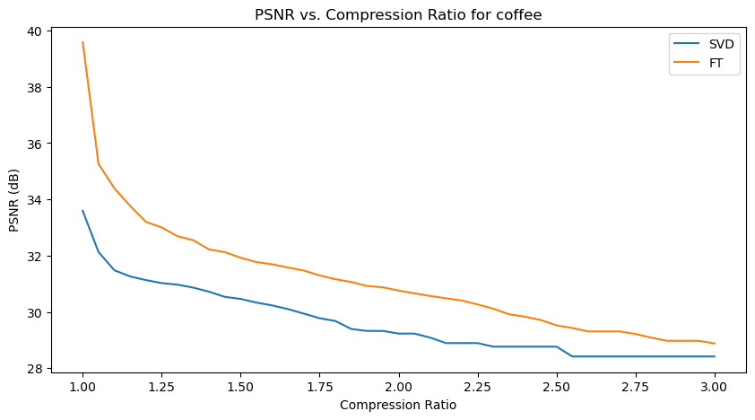
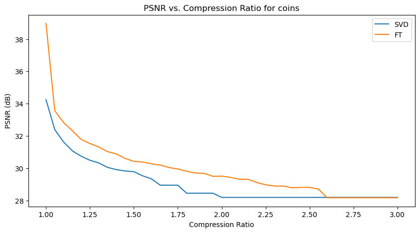
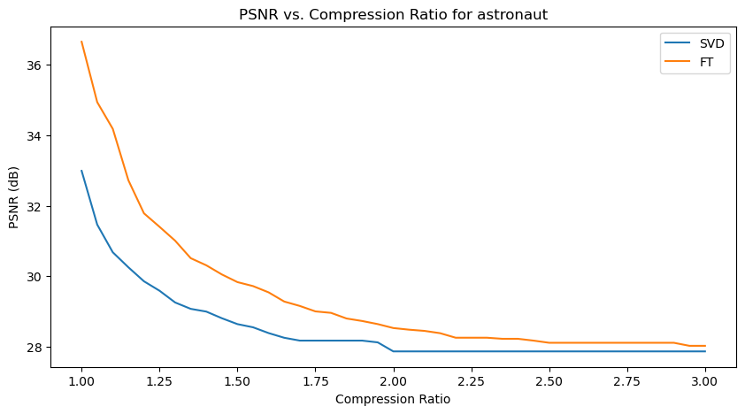
Let’s analyze the PSNR - Compression Ratio plots first:

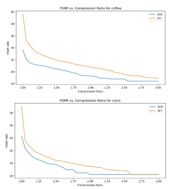
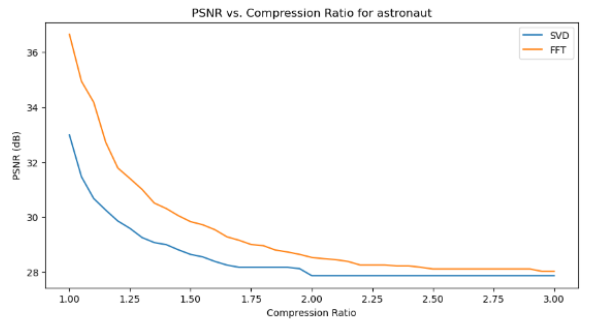
In the above PSNR - Compression Ratio plots, the orange curve represents the FT compressed images, while the blue curve represents the SVD compressed images.

Given the formula of PSNR, having a higher PSNR is favorable for image quality.

We can observe that the FT compression yields consistently greater PSNR values than SVD compression, which implies that FT compressed images generally have a better image quality. This is also supported by our qualitative observation earlier, that FT compressed images generally resemble their original versions better than SVD compressed images.

However, we can also make an interesting observation that for increasing compression ratios, the fall in PSNR for FT is generally steeper than SVD. This might be explained by the fact that as compression ratio increases, FT-images lose high frequency details (fine details) faster, which PSNR is sensitive to. Whereas in SVD compression, only the “least important” singular values are removed first, so the core structure of the image is preserved longer, resulting in a slower drop in PSNR.

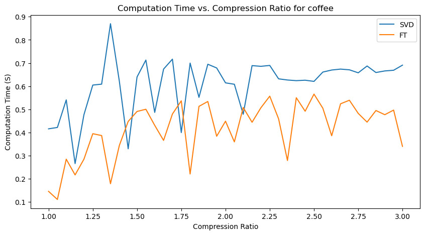
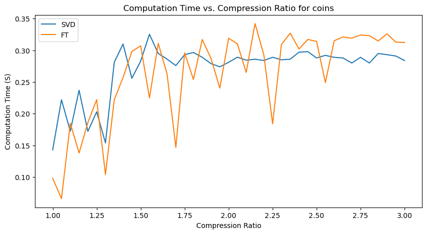
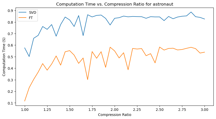
Next, we will analyze the Computation Time - Compression Ratio plots.

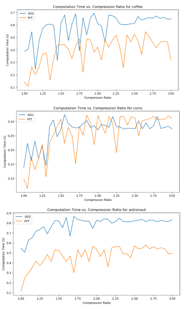
We can observe that there is a general increasing trend in Computation Time as compression ratio increases.

Another important observation is that SVD compression time is generally greater than FT compression times, with the exception for the “coins” image, where they seem roughly similar.

An interesting observation is also that there are many unexpected “spikes” and “drops” in Computation Time as we span the range of possible compression ratios. Upon analysis, this may actually be attributed to two factors:

1. Effect of image content - for images with a lot of structures, like “coffee” (wood texture background) and “coins” (metal engraving texture within the coins), the compression algorithms may take longer at certain compression levels to determine which details to keep and discard.

2. Imperfect resource management (memory management and CPU load) on my computer - each iteration creates and stores new versions of compressed images, which may affect memory management and occasionally cause spikes in computation time from the allocation and deallocation of large matrices.

However, the general increasing trend in Computation Time, and relative demand on Computation Time for SVT and FT are observable nonetheless!

6. Conclusion

From the qualitative and quantitative analysis of our images, we can conclude that:

1. Qualitatively, FT-compressed images resemble their original versions with greater quality than SVD-compressed images. Even when both types of compressed images have visible defects, the “ringing effect” of FT seems more organic than the stark “orthogonal lines” of SVD (especially for images with natural subjects).

2. FT-compressed images have a greater overall PSNR than SVD-compressed images, so FT-compressed images look better.

3. FT-compressed images have a lower overall computation time than SVD-compressed images, so FT compression is also more efficient.

To conclude our findings for this project, the Fourier Transform algorithm is preferred for image compression over Singular Value Decomposition.

Moving forward, there are also some interesting avenues for further research. One promising direction is to extend the analysis to RGB images instead of only grayscale, allowing us to explore the effects of SVD and FT compression in the color domain.

Given that human perception tends to be more sensitive to changes in luminance than chrominance, this investigation could reveal nuanced insights into how these compression algorithms impact color fidelity and visual quality.

Finally, it would also be valuable to assess the performance of these compression techniques on a wider variety of image types, especially images with high-resolution and diverse subjects.