A Revision of Linear Algebra
I share my revision on basic linear algebra, and attempt to construct a geometric intuition based on 3B1B's teaching material.
This blog post is intended to be a quick revision of some linear algebra fundamentals to reference when needed. These notes won’t be the most rigorous or formal, but hopefully they will be useful in quickly rebuilding a geometric intuition when needed.
Vector notation
We express vectors in this notation: $[a, b]$ - in this case, to express a 2D vector.
Scalars
When a vector is multiplied by a number, it is “scaled” by the magnitude of that number. So, we often use the term “scalar” interchangeably for numbers.
Basis Vectors
Given a conventional 2D graph for example, we have basis vectors $\hat{j}$ and $\hat{k}$, which are aligned with the y-axis and x-axis respectively. Our coordinate values scale our basis vectors, and our final output vector is the sum of the two scaled basis vectors.
Vectors as Linear Combinations
Let’s say we are given two different vectors $\vec{V}$ and $\vec{W}$. We scale each vector, then sum them together, producing something like $a\vec{V}$ + $k\vec{W}$. This output is called a “Linear Combination” of vectors $\vec{V}$ and $\vec{W}$.
Span
For the linear combination above, $a\vec{V}$ + $k\vec{W}$, let’s say we can vary scalars $a$ and $b$ as we please. The set of all possible linear combinations we can produce is called the “Span” of the vectors $\vec{V}$ and $\vec{W}$.
If our two 2D vectors $\vec{V}$ and $\vec{W}$ are not parallel, we can imagine that the span covers the entire 2D plane. Now, what if we had three 3D vectors, and the third vector specifically lies outside of the span of the first two vectors? Then, our three 3D vectors would span the entire 3D space.
Now, what if the third 3D vector lies in the same direction as one of the other two 3D vectors? Or, what if the third 3D vector lies in the span of the first two 3D vectors? Then, we could literally remove the third 3D vector, without affecting the span of the original three 3D vectors. Thus, we can say that these vectors are “Linearly Dependent”.
Linearly Independent Vectors
If every vector in a set of vectors increases the span of the set, each vector in the set is linearly independent. In other words, to achieve linear independence, no vector in the set can be expressed as a linear combination of the others.
Linear Transformations
Transformation is a fancy word for “function”. It is something that takes in an input, and produces an output. Linear transformations have two properties:
- All straight lines must remain straight lines without curvature, after transformation
- The origin must remain fixed.
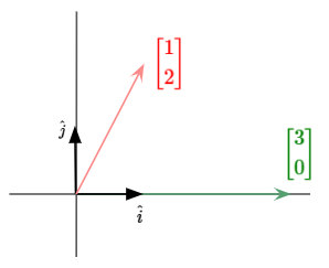
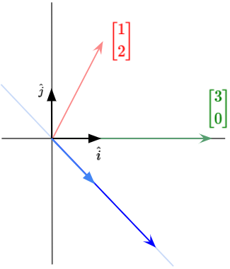
For example, let’s say we have $\vec{V}$ = $-1\vec{i}$ + $2\vec{j}$. If we transform $\vec{i}$ to $[-1,2]$ as its new basis, and $\vec{j}$ to $[3,0]$ as its new basis, our vector $\vec{V}$ is transformed into $[5,2]$.
Matrix Transformations
Let’s generalize the concept of a linear transformation.
Let’s say you have a vector $\begin{bmatrix} x \cr y \end{bmatrix}$, and you want to transform $x$ by $\begin{bmatrix} a \cr c \end{bmatrix}$ and $y$ by $\begin{bmatrix} b \cr d \end{bmatrix}$.
We can express these transformations mathematically like so:
We can see that the column containing $[a,c]$ has transformed our $x$ basis, and the column containing $[b,d]$ has transformed our $y$ basis.
Recall that a Linear Transformation is defined by where it moves the basis vectors of the space. Therefore, we must also think of Matrix Transformations as a certain transformation of the space.
Determinant
Naturally, we would also want to measure how much a matrix multiplication operation (a linear transformation of our basis vectors) actually affects the area of a given region, whether by stretching or compressing it.
For example, we can see that $\begin{bmatrix} 3 & 0 \cr 0 & 2 \end{bmatrix}$ $\begin{bmatrix} 1 \cr 1 \end{bmatrix}$ would produce the following:
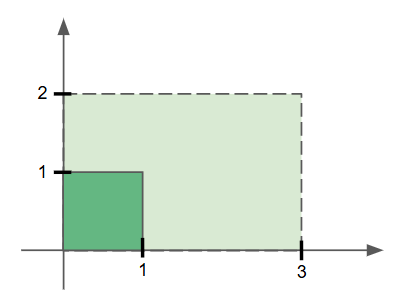
We see that the original unit square area covered by our basis vectors is scaled from a $1$ ${unit}^2$ to $6$ ${unit}^2$ region.
This tells us that any square or rectangle will also be scaled by a factor of 6 after this matrix multiplication operation. However, this scaling also applies for other irregular shapes too.
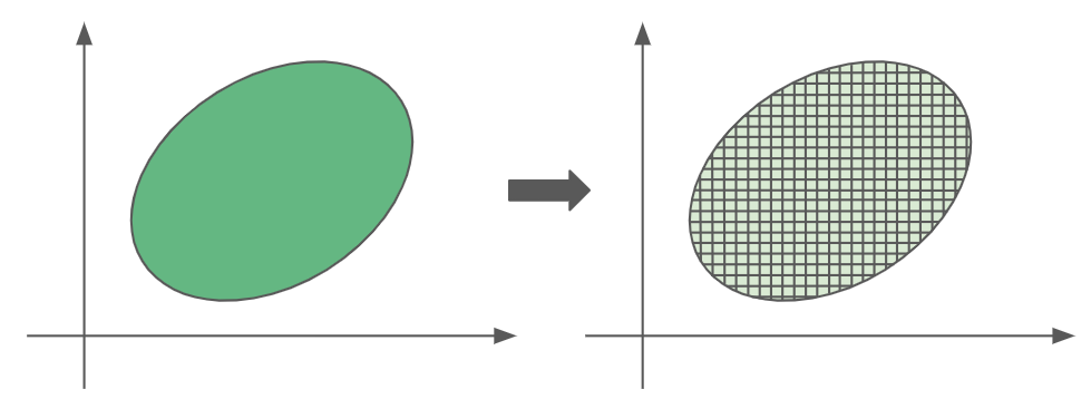
For instance, we can break down our irregular shape into many infinitesimally small squares. We know for a fact that each of these squares will scale by a factor of 6, so the entire irregularly shaped region will scale accordingly too.
This scaling factor arising from a matrix multiplication is called the determinant of the matrix.
Additional Properties of Determinants
Let’s explore some interesting properties about determinants by answering some questions about them:
What happens when the determinant is zero?
Well, having a zero determinant means your scaling factor is zero, so your final shape has an area of zero. For example, if the determinant of a 2D transformation matrix is zero, it ‘squishes’ all the 2D space into a single line or point, resulting in a zero area. More formally, we can say that a zero determinant means a matrix is not full rank, so the matrix multiplication causes the output to lose at least one dimension.
Finally, we should also note that a matrix with a zero-valued determinant is called a Singular Matrix.
Okay, then what happens when the determinant is negative?
In that case, the original input region is still scaled by the magnitude of the determinant, but the region is also flipped. It may be hard to visualize, so let’s build our intuition this way: Given a pair of basis vectors $\hat{i}$ and $\hat{j}$, we’ll shear the region produced by these basis vectors by rotating basis vector $\hat{i}$ clockwise.
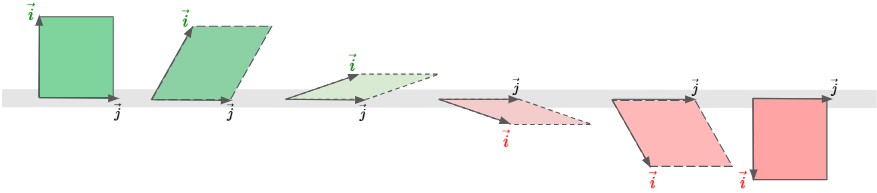
Now, let’s think about how the value of determinant will change as we rotate the $\hat{i}$ basis vector.
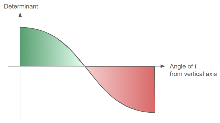
When comparing positive and negative determinant values of the same magnitude, we see that the regions are simply flipped images of each other. Therefore, a negative determinant value does both scaling and flipping of an input region.
What about determinants in a 3x3 matrices? Determinants of 3x3 matrices give us the scaling factor of the volume. If the determinant of a 3x3 matrix is zero, this means space is squished into something with 0 volume, like a flat plane, line or point.
Let's see how linear algebra can be used to solve simultaneous linear equation problems:
If the determinant of $A$ is not zero, there is only one possible value of vector $\vec{x}$ that can be transformed into vector $\vec{v}$. We can visualize this by reversing the transformation that happened to vector $\vec{v}$. This operation is called an inverse transformation, such as $A^{-1}(\vec{v})$.
When matrix $\vec{A^{-1}}$ is multiplied with matrix $A$, such that we have $A^{-1}(A)$, we should got back a matrix that produces a transformation that does nothing. This matrix is called an identity matrix, and it looks something like this: ${\begin{bmatrix} 1 & 0 \cr 0 & 1 \end{bmatrix}}$.
So, we solve for $\vec{x}$ by applying $(A^{-1}A) \vec{x} = A^{-1} \vec{v}$.
Geometrically, this means we’re playing the transformation in reverse for $\vec{v}$.
But, what happens if the determinant of $A$ is zero for $A \vec{x} = \vec{v}$? In that case, there is no inverse. During the ‘squishing’, we lose information about the original points that are mapped onto the lower dimensional subspace. There is no function that can take a single line input (for example) and reconstruct the original 2D plane accurately (except for some particular edge cases).
In summary, a matrix with a zero-valued determinant is not invertible.
Rank
We may also notice that some zero-determinant cases are more restrictive than others. For a 3x3 matrix, it’s a lot harder for a solution to exist if it is squished into a line, rather than being squished into a plane.
We have some new language to use in describing these zero-determinant cases:
- If the output is a point, it is a 0-dimensional output, so the matrix has a rank 0.
- If the output is a line, it is a 1-dimensional output, so the matrix has a rank 1.
- If the output is a plane, it is a 2-dimensional output, so the matrix has a rank 2.
- and so on…
Column Space
The set of all possible outputs for your matrix (whether it’s a line, plane, 3D volume, etc.) is the column space of your matrix.
The columns of a matrix tell you where your basis vectors are transformed to. Then, the span of those transformed basis vectors gives you the space of all possible outputs. So, the column space is the span of the columns in a matrix.
In a sense, the rank describes the maximum number of linearly independent columns in your matrix. It also describes the number of dimensions covered by your column space.
When rank is at maximum value for a matrix, we call the matrix “full rank”. Full rank matrices will only map the zero vector to origin, while non-Full Rank matrices will map other vectors to origin.
Dot Products
The dot product between two vectors is defined by the projection of one vector onto the other. More specfically, Dot products are the product of the $\text{(Projection of W on V)} \centerdot (V)$.
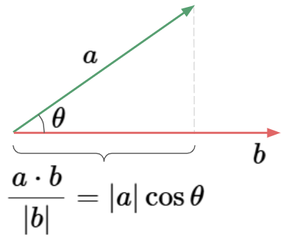
The formula for dot product is like so:
We can also notice an interesting duality between a matrix-vector product and a dot product:
Therefore, we can see that computing the projection transformation for arbitrary vectors in space is computationally identical to taking a dot product with the matrix $\hat{U}$.
This is why taking the dot product with a unit vector can be interpreted as projecting a vector onto the span of that unit vector and taking the length. Then, in the case of taking the dot product with a non-unit vector, we first project onto the span of the non-unit vector, then scaling up the length of projection by the length of that vector.
So, the dot product now becomes a very useful geometric tool for understanding projections and for testing whether two vectors tend to point in the same direction.
But at a deeper level, we now see that dotting two vectors together is a way to translate one of them into the world of transformations.
Cross Products
Given two different 3D vectors, the cross product operation is something that combines the two different 3D vectors to get a new 3D vector.
Consider the parallelogram formed by the two 3D vectors that we are crossing together. The area of this parallelogram is going to play a big role in the cross product.
It was mentioned earlier that the cross product is a vector. This new vector’s length will be the area of the parallelogram, and the direction of that new vector is going to be perpendicular to that parallelogram.
How do we decide which direction the normal vector (or cross product) should point? We can use the right-hand rule to solve for that.
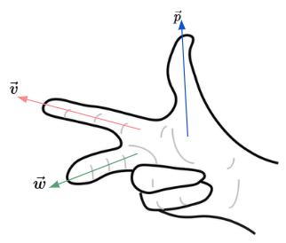
We align the vector $\vec{v}$ to our index finger, and the vector $\vec{w}$ to our middle finger. Then, pointing our thumb up, we now see that the cross product $\vec{p}$ points in the same direction as our thumb.
For cross product computations, we usually use the following formula:
Eigenvectors & Eigenvalues
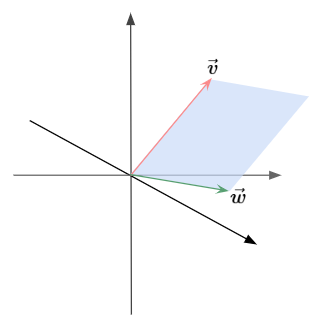
During a linear transformation, let’s say with the matrix $\begin{bmatrix} 3 & 1 \cr 0 & 2 \end{bmatrix}$, the $\hat{i}$ basis vector is moved to $\begin{bmatrix} 3 \cr 0 \end{bmatrix}$ while the $\hat{j}$ basis vector is moved to $\begin{bmatrix} 1 \cr 2 \end{bmatrix}$.
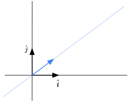
Let’s try to understand what this transformation does. To do that, we will focus in on what it does to one particular vector. Let’s also imagine the span of that vector. We have illustrated an example vector in blue below.
During the transformation, most vectors will get knocked off their span.
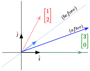
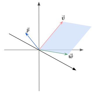
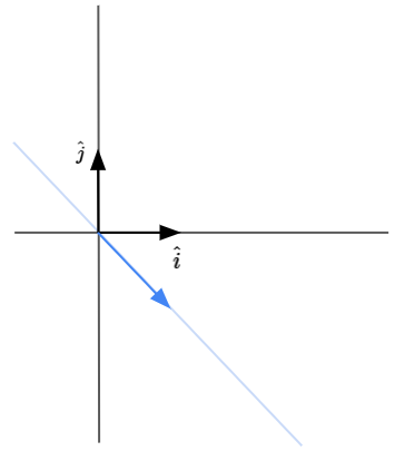
It would seem pretty unlikely for the vector land along the exact same span after transformation. However, there are some vectors that do remain in their own span. Given the example matrix above, the vector $\begin{bmatrix} 1 \cr -1 \end{bmatrix}$ actually remains in its own span during the transformation, as seen below.
This means that for some particular vectors, the effect of the linear transformation is just to stretch or compress it.
These vectors are called the Eigenvectors of that particular linear transformation.
Each of them have what’s called an Eigenvalue, which represents the stretching/compressing scaling factor of that transformation on that eigenvector.
Mathematically, for a transformation matrix $A$, the eigenvectors and eigenvalues are defined as:
For simpler computations, we solve for the eigenvectors and eigenvalues like so:
To find a non-zero solution for $\vec{v}$, we need to solve for the determinant of $(A- \lambda I)$ = 0. This is because $(A- \lambda I)\vec{v} = 0$ means every non-zero vector $\vec{v}$ lying in the null space of matrix $(A- \lambda I)$ is squished to zero. So, we need $det(A-\lambda I)$ to hold.
Let’s now move on to a more higher-level view of this topic. We learned that the eigenvector describes directions in the space that remain invariant under a particular transformation (defined by the matrix). Why is this such an important concept to master?
In the broader context of linear algebra, thinking of transformations as linear transformations of our basis vectors makes us very dependent on a particular coordinate system. Instead, we could find the eigenvectors and eigenvalues to understand a transformation, independent of a specific coordinate system.
Additional tidbit: imagine a 3D rotation happening due to a transformation. If you know the eigenvector of that transformation, you have found the axis of the rotation operation! (Also, since this is a pure rotation operation, the eigenvalue would be 1)
References
Please watch 3B1B’s excellent series on Linear Algebra