How I learned the Fourier Transform intuitively

So I got curious about the topic of image compression one afternoon, and realized I needed to understand the Fourier Transform. The Fourier Transform extends the Fourier Series to handle non-periodic signals, and “transforms” the input signal from the time/spatial domain to the frequency domain. This allows us to analyze a given signal from a frequency perspective.

Here’s a compilation of my learning notes throughout this journey.

$~ \\$

Let’s begin with a small flowchart for how I moved step-by-step towards understanding this topic:

$\text{1. Understand the Fourier Series} \\ \Downarrow \\ \text{2. Express Fourier Series in Euler Form} \\ \Downarrow \\ \text{3. Generalize Fourier Series to non-periodic functions, then obtain Fourier Transform} \\$

$~ \\$

Let’s break this blog post down into 3 main chapters based on the points above.

1. What’s the core idea of the Fourier Series?

Let’s say we want to work with periodic functions, whereby $f(t + T) = f(t)$. We will use $2\ pi $-periodic functions for now.

Now, let’s say we have a square wave, which is $2 \pi$-periodic, like so:

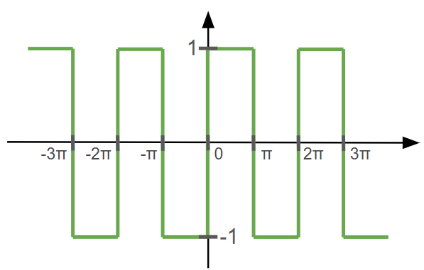
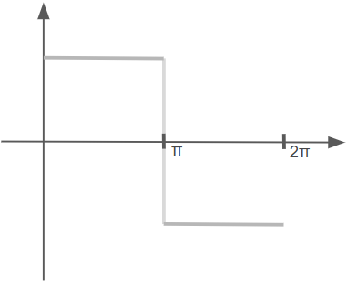
Let’s make things cleaner by zooming in on just one period here:

What if we overlay a single sine wave, $\frac{4}{\pi} \sin x$, over the square wave? No worries about the $\frac{4}{\pi}$ term, it’s just a scaling factor to keep things clean later.

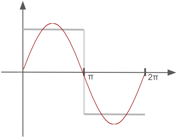
We see that it forms somewhat of a (poor) approximation of the square wave.

Now, let’s see what happens if we add in another sine function, $\frac{4}{\pi} \cdot \frac{1}{3} \sin (3x)$.

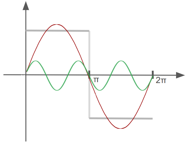
The $(3x)$ term in the second sine function means that the function is oscilating much faster, in a way that “destructively interferes” with the original sine function.

This then produces the following improved approximation:

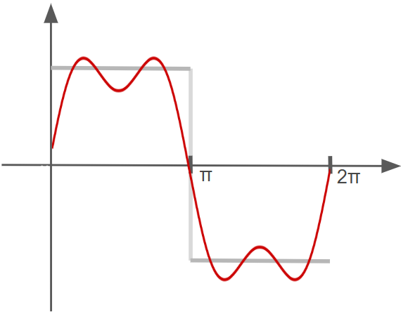
Looking good! Now, if we keep at this, adding $\frac{4}{\pi}\frac{1}{5} \sin(5x)$, $\frac{4}{\pi}\frac{1}{7}\sin(7x)$, and so on, the approximation should improve. Here’s what a further iteration might look like:

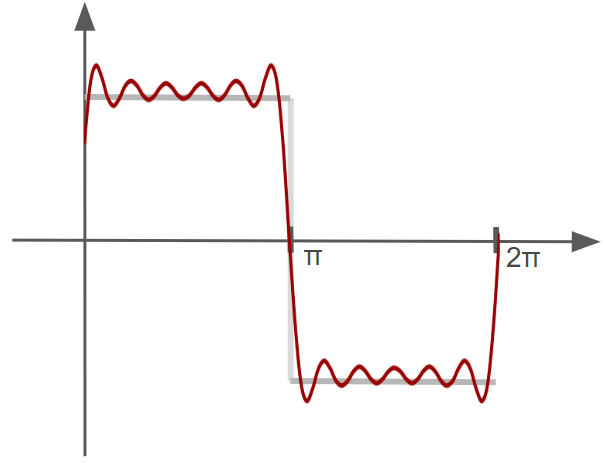
Now, the approximation looks much better! The approximation above is defined as:

$\boxed{\frac{4}{\pi} \displaystyle\sum_{n=1,3,5...}^{11} \frac{\sin (nx)}{n}}$

We stopped at $n = 11$, but this summation could be extended to $n \to \infty$ to get an even better approximation.

So the big idea of a fourier series is that we take in a function, and by adding up a whole bunch of trigonometric terms of different frequencies, we can obtain an equivalent approximation to the input function.

$~ \\$

Moving on, let's substantiate our idea of a fourier series a little. Now we’ll also consider the addition of cosine terms, to allow us to approximate more types of input functions.

So, let’s say our input function $f(t)$ has a period of $2 \pi$, using our idea of the Fourier Series, we would express $f(t)$ as:

$\boxed{f(t) = \frac{a_0}{2} + \displaystyle\sum_{n=1}^{\infty} a_n \cos(nt) + \displaystyle\sum_{n=1}^{\infty} b_n \sin(nt)}$

For now, please ignore the $\frac{a_0}{2}$ component, it is a mathematical convention that we will explore later.

$~ \\$

Given this formulation above, let's revisit the example of our "odd-functional" square wave above. We know that we can approximate the square wave by:

$\boxed{f(t) = \frac{4}{\pi} \displaystyle\sum_{n=1,3,5...}^{\infty} \frac{\sin (nx)}{n}}$

Since all the $\cos$ terms are empty, we know that $a_n = 0$. For $b_n$, if $n$ is odd-numbered, $b_n = \frac{4}{\pi} \cdot \frac{1}{n}$. If $n$ is even-numbered, $b_n = 0$.

$~ \\$

Next, let's generalize our understanding of the Fourier Series more, by including non-2π periodic functions.

Given a function $f(t)$ defined on some interval $[-L, L)$, we would now have:

$\fcolorbox{orange}{white}{$f(t) = \frac{a_0}{2} + \displaystyle\sum_{n=1}^{\infty} a_n \cos(\frac{\pi}{L} nt) + \displaystyle\sum_{n=1}^{\infty} b_n \sin(\frac{\pi}{L}nt)$}$

Notice the “stretching factor” of $\frac{\pi}{L}$ inside the cosine and sine terms? This maps the interval of $[-L,L)$ into $[- \pi, \pi)$, which allows our basis functions to match the new periodicity.

$~ \\$

Next, there remains another fundamental question: how do we find $a_0$, $a_n$ and $b_n$? Let's find out how to compute them.

Let’s begin with three core integrals related to the concept of functional orthogonality:

$\int_{0}^{2\pi} \sin(mt) \sin(nt) \space dt = \begin{cases} 0 &\text{if } m \ne n \\ \pi &\text{if } m = n \end{cases} \\ ~ \\ \int_{0}^{2\pi} \cos(mt) \cos(nt) \space dt = \begin{cases} 0 &\text{if } m \ne n \\ \pi &\text{if } m = n \end{cases} \\ ~ \\ \int_{0}^{2\pi} \cos(mt) \sin(nt) \space dt = 0 \space \text{for any m,n}$

Let’s see how we can use the above knowledge to decompose our $f(t)$ into its constituent sinusoidal functions.

1. Finding coefficient $b_n$

Firstly, let’s multiply $f(t)$ with $\sin(mt)$ and integrate, but do this to both sides of the equation:

$\int_{0}^{2\pi} f(t) \sin(mt) \space dt =\int_{0}^{2\pi} (\frac{a_0}{2} + \displaystyle\sum_{n=1}^{\infty} a_n \cos(nt) + \displaystyle\sum_{n=1}^{\infty} b_n \sin(nt)) \sin(mt) \space dt \\ ~ \\ \Downarrow \\ ~ \\ = \int_{0}^{2\pi} (\textcolor{red}{\cancel{\frac{a_0}{2}}} + \displaystyle\sum_{n=1}^{\infty} a_n \textcolor{red}{\cancel{\cos(nt)}} + \displaystyle\sum_{n=1}^{\infty} b_n \sin(nt)) \sin(mt) \space dt \\ ~ \\ \Downarrow \\ ~ \\ = \int_{0}^{2\pi} b_m \sin(mt) \sin(mt) \space dt \\ \text{* where n = m. For all other n, sin(nt)=0} \\ ~ \\$

To clean things up, we can show that:

$\int_{0}^{2\pi} f(t) \sin(mt) \space dt = \int_{0}^{2\pi} b_m \sin(mt)^2 \space dt = b_m(\pi) \\ ~ \\$

Therefore, we found that:

$\fcolorbox{orange}{white}{$b_m = \frac{1}{\pi} \int_{0}^{2\pi} f(t) \sin(mt) \space dt$} \\ ~\\ \text{Since m is a variable, we now know how to find all values of coefficient b.} \\ ~ \\$

2. Finding coefficient $a_n$

Now, let’s multiply the expression for $f(t)$ with $\cos(mt)$ and integrate.

$\int_{0}^{2\pi} f(t) \cos(mt) \space dt =\int_{0}^{2\pi} (\textcolor{red}{\cancel{\frac{a_0}{2}}} + \displaystyle\sum_{n=1}^{\infty} a_n \cos(nt) + \displaystyle\sum_{n=1}^{\infty} b_n \textcolor{red}{\sin(nt)}) \cos(mt) \space dt \\ ~ \\ \Downarrow \\ ~ \\ = \int_{0}^{2\pi} a_n \cos(mt) \cos(mt) \space dt \\ ~ \\ \Downarrow \\ ~ \\ = a_m(\pi)$

In summary, we can say that:

$\fcolorbox{orange}{white}{$a_m = \frac{1}{\pi} \int_{0}^{2\pi} f(t) \cos(mt) \space dt$} \\ ~ \\$

3. Finding coefficient $a_0$

Finally, let’s multiply both sides of the $f(t)$ equation by 1, and integrate:

$\int_{0}^{2\pi} f(t) \cdot 1 \space dt =\int_{0}^{2\pi} (\frac{a_0}{2} + \displaystyle\sum_{n=1}^{\infty} a_n \textcolor{red}{\cancel{\cos(nt)}} + \displaystyle\sum_{n=1}^{\infty} b_n \textcolor{red}{\cancel{\sin(nt)}}) \cdot 1 \space dt \\ ~ \\ \Downarrow \\ ~ \\ = a_0(\pi)$

In summary, we can say that:

$\fcolorbox{orange}{white}{$a_0 = \frac{1}{\pi} \int_{0}^{2\pi} f(t) \cdot 1 \space dt$} \\ ~ \\$

Fourier Series Convergence and Chapter 1 Summary

Nice! So far, we’ve understood how the Fourier Series can be decomposed into sinusoidal components, and we’ve shown how the coefficients are derived. There remains one final question: How do we know if a particular fourier series (sum of sinusoidal components) actually converges?

We can refer to the Fourier Convergence Theorem, which states that if $f$ and $f’$ are piecewise continuous on $[-L,L)$, $f(t) = \frac{a_0}{2} + \displaystyle\sum_{n=1}^{\infty} a_n \cos(\frac{\pi}{L} nt) + \displaystyle\sum_{n=1}^{\infty} b_n \sin(\frac{\pi}{L}nt)$ will converge. If there is a discontinuity, the fourier series converges to midpoint on the discontinuity.

2. Expressing the Fourier Series in Complex Form

In this chapter, we are going to rewrite the Fourier Series formula in its complex form. This will help us in future steps when we are formulating the Fourier Transform.

Let’s begin by stating Euler’s Formula and its derivative trigonometric identities:

$\begin{aligned} e^{i \theta}&=\cos \theta + i \sin \theta \\ e^{-i \theta}&=\cos \theta - i \sin \theta \\ ~\\ cos \theta &= \frac{1}{2}(e^{i \theta}+e^{-i \theta}) \\ sin \theta &= \frac{1}{2i}(e^{i \theta}-e^{-i \theta}) \\ \end{aligned} ~ \\$

Our Fourier Series will have a period defined as $T$. Let’s also define a new variable called Angular Frequency ($\omega$), which is defined as:

$\omega = \frac{2\pi}{T} \\ ~ \\$

Now let’s begin re-framing our Fourier Series expression in complex form:

$\begin{aligned} f(t) &= \frac{a_0}{2} + \displaystyle\sum_{n=1}^{\infty}[ a_n \cos(\frac{2\pi nt}{T}) + b_n \sin(\frac{2\pi nt}{T})] \\ &= \frac{a_0}{2} + \displaystyle\sum_{n=1}^{\infty}[ a_n \cos(\omega_0 nt) + b_n \sin(\omega_0 nt)] \\ &= \frac{a_0}{2} + \displaystyle\sum_{n=1}^{\infty}[ \frac{a_n}{2} (e^{i \omega_0 nt} + e^{-i \omega_0 nt}) + \frac{b_n}{2i} (e^{i \omega_0 nt} - e^{-i \omega_0 nt})] \\ &= \frac{a_0}{2} + \displaystyle\sum_{n=1}^{\infty}[ (\frac{a_n}{2}+\frac{b_n}{2i}) (e^{i \omega_0 nt}) + (\frac{a_n}{2}-\frac{b_n}{2i}) (e^{-i \omega_0 nt}) ] \\ &= \frac{a_0}{2} + \displaystyle\sum_{n=1}^{\infty}[ \frac{1}{2} (a_n - i b_n) (e^{i \omega_0 nt}) + \frac{1}{2} (a_n + i b_n) (e^{-i \omega_0 nt}) ] \\ &= \frac{a_0}{2} + \displaystyle\sum_{n=1}^{\infty}[ C_n (e^{i \omega_0 nt}) + C_n^* (e^{-i \omega_0 nt}) ] \\ &= C_0 + \displaystyle\sum_{n=1}^{\infty}[ C_n (e^{i \omega_0 nt})] +\displaystyle\sum_{n=-1}^{-\infty} [ C_n (e^{i \omega_0 nt}) ] \space \color{red}\circledast \\ &= \displaystyle\sum_{n=-\infty}^{\infty}[ C_n (e^{i \omega_0 nt})] \\ \end{aligned} ~ \\ ~ \\ \text{whereby:} \begin{array}{c:c:c} C_0 = \frac{a_0}{2} & C_n = \frac{a_n - i b_n}{2} & C_n^* = \frac{a_n + i b_n}{2} \end{array} \\ ~ \\$

You may have noticed that we pulled a trick in the line labelled $\color{red}\circledast$, where we basically claimed that $C_n^* = C_{-n}$. Here’s a quick demonstration:

$\begin{aligned} \text{For } C_n &= \frac{a_n - i b_n}{2} \text{ ,} \\ C_{-1} &= \frac{a_{-1} - i b_{-1}}{2} \\ &= \frac{\int f(x)\cos(-x) - i \int f(x) \sin(-x)}{2} \\ &= \frac{\int f(x)\cos(x) + i \int f(x)\sin(x)}{2} \\ ~ \\ \end{aligned}$

$\begin{aligned} \text{For } C_n^* &= \frac{a_n + i b_n}{2} \text{ ,} \\ C_1^* &= \frac{a_{1} + i b_{1}}{2} \\ &= \frac{\int f(x)\cos(x) + i \int f(x)\sin(x)}{2} \\ ~ \\ \end{aligned}$

Hence, $C_n^* = C_{-n}$.

Now, let’s summarize our findings for this chapter. We re-wrote our Fourier Series in complex form, such that:

$\fcolorbox{red}{white}{$f(t) = \frac{a_0}{2} + \displaystyle\sum_{n=1}^{\infty}[ a_n \cos(\frac{2\pi nt}{T}) + b_n \sin(\frac{2\pi nt}{T})] \\ = \displaystyle\sum_{n=-\infty}^{\infty}[ C_n (e^{i \omega_0 nt})]$}$

3. Informal Derivation of Fourier Transform from non-periodic Fourier Series

So far, we’ve been working with an input function $f(t)$ which is defined to have a period $T$. In the previous chapter, we found that we can express $f_T(t)$ as $\displaystyle\sum_{n=-\infty}^{\infty}[ C_n (e^{i \omega_0 nt})]$, where $\omega_0 = \frac{2\pi}{T}$.

Notice how we previously named the variable $\omega$ as “Angular Frequency”? For the fourier series expression defined above, there are harmonics of frequency $n \omega_0 = n \cdot \frac{2\pi}{T}$ present, for which $n = 0, \pm 1, \pm 2, …$.

This is because a periodic function like $f_T(t)$ repeats itself every period $T$, which means the frequency components must align with the periodicity. So, the Fourier Series only consists of sinusoidal components whose frequencies are multiples of the fundamental frequency $\omega_0 = \frac{2\pi}{T}$.

These harmonic frequencies are separated by $n \omega_0 - (n-1) \omega_0 = \omega_0 = \frac{2\pi}{T}$. Let’s rewrite this frequency separation as $\triangle \omega$, whereby $\triangle \omega = \omega_0$.

Let’s say we increase the variable period $T$. When $T \uparrow$, $\omega_0 \downarrow$. So, for a non-periodic function with $T \to \infty$, we have $\triangle \omega \to 0$. As a result, the frequency components are no longer separated by a finite interval $\triangle \omega$, and instead form a continuous spectrum of frequencies. This means our ‘non-periodic fourier series’ now contains all frequency harmonics rather than just multiples of $\omega_0$.

Let’s see this in action:

Firstly, let’s find an expression for $C_n$:

$C_n = \frac{1}{T} \int_{\frac{-T}{2}}^{\frac{T}{2}} f_T(t) \cdot e^{-in\omega_0 t} \space dt \\ ~ \\$

Next, we will substitute $\frac{1}{T}$ for $\frac{\omega_0}{2 \pi}$, and substitute this, along with the expression for $C_n$ into the expression for $f_T(t)$.

This gives us:

$f_T(t) = \displaystyle\sum_{n=-\infty}^{\infty} [\frac{\omega_0}{2\pi} \int_{\frac{-T}{2}}^{\frac{T}{2}} f_T(t) e^{-in\omega_0 t} \space dt] \cdot e^{in\omega_0 t} \\ ~ \\$

Let’s mentally substitute $\omega_0$ for $\triangle \omega$. Notice now that as $\triangle \omega \to 0$, the term involving the infinite sum over the discrete frequencies $n \omega_0$ helps form a Riemann Sum! So, we can replace the infinite sum over the discrete frequencies by an integral over all frequencies. In our mathematical working, we will simply replace all $(n\omega_0)$ with a general frequency variable, $\omega$.

Thus, we will obtain the following double integral representation form:

$\begin{aligned} f(t) &= \displaystyle\sum_{n=-\infty}^{\infty} [ [\frac{1}{2\pi} \int_{\frac{-T}{2}}^{\frac{T}{2}} f_T(t) e^{-in\omega_0 t} \space dt] \cdot e^{in\omega_0 t}] \\ &= \int_{-\infty}^{\infty} [\frac{1}{2\pi} \int_{-\infty}^{\infty} f(t) e^{-i \omega t} \space dw] \\ ~ \\ \end{aligned}$

The inner integral over all $t$ will give a resulting function only dependent on $\omega$, which we will define as $F(\omega)$. This allows us to simplify the expression a lot. We thus obtain:

$\fcolorbox{red}{white}{$f(t) = \frac{1}{2\pi} \int_{-\infty}^{\infty} F(\omega) e^{i \omega t} \space dw$} \\ ~ \\ \text{and} \\ ~ \\ \fcolorbox{red}{white}{$F(\omega) = \int_{-\infty}^{\infty} f(t) e^{-i \omega t} \space dt$} \\ ~ \\$

$F(\omega)$ is called the Fourier Transform of function $f(t)$, while $f(t)$ is called the Inverse-Fourier-Transform of $F(\omega)$. We just (informally) derived the Fourier Transform from the Fourier Series!

We can see why it is called the Fourier “Transform”, because it transforms an input function from the time/spatial domain (eg. $t$) into the frequency domain ($\omega$).

Next, let’s gain a deeper intuition for what the Fourier Transform does.

Understanding the Fourier Transform intuitively

So we ended the previous chapter by showing how the Fourier Transform of an input function $f(t)$ is $F(\omega) = \int_{-\infty}^{\infty} f(t) e^{-i \omega t} \space dt$. Let’s now simplify the scary-looking exponential term and gain a deeper understanding for how the Fourier Transform works.

Using $e^{-i\omega t} = \cos(-\omega t) + i \sin(-\omega t) = \cos(\omega t) - i \sin(\omega t)$, we have:

$\begin{aligned} ~ \\ F(\omega) &= \int_{-\infty}^{\infty} f(t) e^{-i \omega t} \space dt \\ &= \int_{-\infty}^{\infty} f(t) [\cos(\omega t) - i \sin(\omega t)] \space dt \\ &= \int_{-\infty}^{\infty} f(t) \cos(\omega t) \space dt -i \int_{-\infty}^{\infty} f(t) \sin(\omega t) \space dt \\ ~ \\ \end{aligned}$

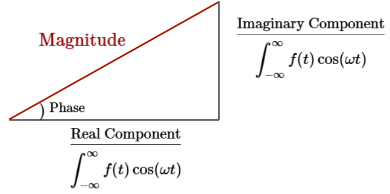
So, given an input function $f(t)$, multiply your function with a sine and cosine curve of the same arbitrary angular frequency. The area under both of those curves is what the integral tells us.

The magnitude of the area is found using the real and imaginary component of the complex number shown in the above working. But more specifically, the magnitude of that complex number is the magnitude of the Fourier Transform at that specific $\omega$, and the angle is the phase.

$~ \\$

Let’s work through an example!

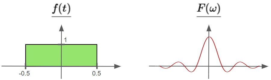
Given an input rectangular function $f(t)$, here’s how it looks beside its associated Fourier Transform $F(\omega)$:

$~ \\$

Let’s proceed to find $f(t) \cos (\omega t)$ and $f(t) \sin (\omega t)$ separately. Then, we will find the integral of each component, or basically, the area under their respective curves:

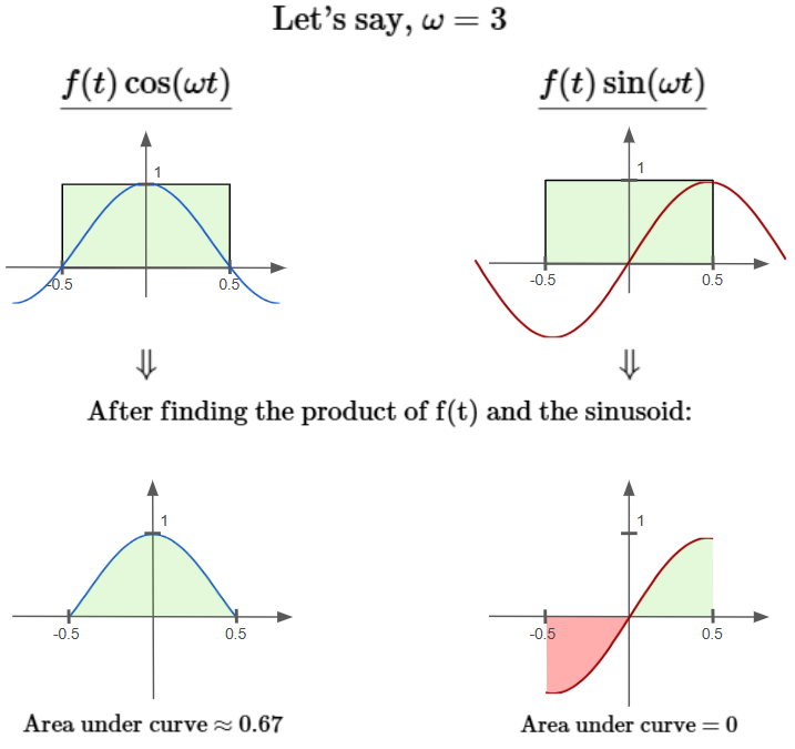
So, at $\omega = 3$, we have $\vert F(\omega) \vert ≈ 0.67$.

$~ \\$

Now, to carry on, we simply have to sweep across all possible values of our variable $\omega$ and find all the associated fourier transform values.

But first, let’s make some observations:

• We notice that for the $f(t) \sin (\omega t)$ component, the area under the graph will always be zero if $f(t)$ is even, since the positive and negative sides cancel out.
• When $\omega = 0$, $\cos (\omega t) = 1$ and $\sin (\omega t) = 0$, so we get back $\int f(t)$, the original area under the graph of $f(t)$.
• When $\omega = 2\pi$, $F(\omega)=0$, because both $\cos (\omega t)$ & $\sin (\omega t)$ have positive and negative regions that cancel out.

$~ \\$

Using these observations above, we can see the plot of $F(\omega)$ naturally forming:

$~ \\$

Okay, moving on, let’s see what happens when we plot a function that is a little more complicated. What if our function was two cosine functions multiplied together?

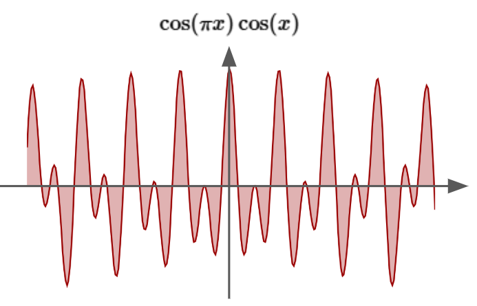
We can observe that the total area under the curve oscillates around some value, between negative and positive.

We can also make another observation: as we vary $k$ and $n$ in $\cos (kx) \cos (nx)$, only when $k = n$ does the graph have all positive values, because we have a $\cos ^2$ graph. This also means the total area under the $\cos ^2$ graph can sum to infinity.

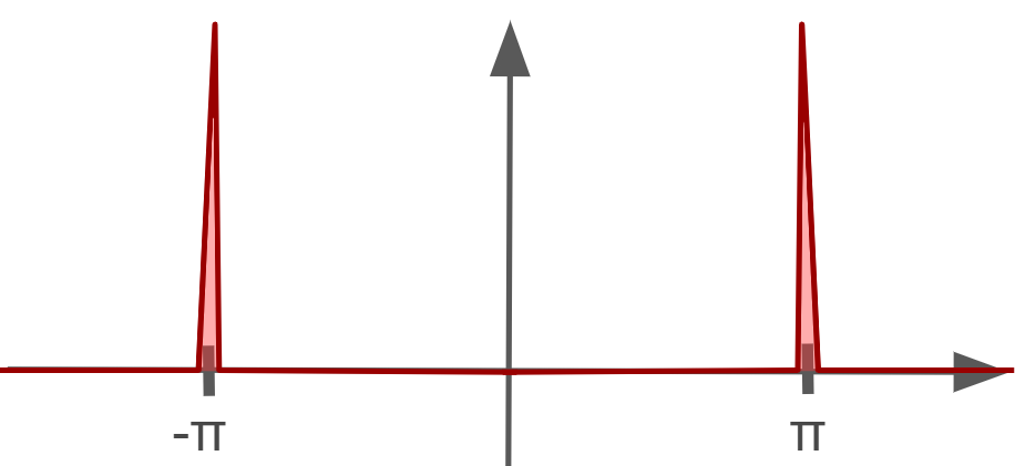
Now, let’s see how the above observations could help us. Now, let’s say our input function $f(t) = \cos (\pi x)$. To find the Fourier Transform of this input, we need to multiply $f(t)$ with $\cos (\omega x)$ and $\sin (\omega x)$, then find the areas of those products.

Let’s use another two observations:

• $\cos (\pi x) \sin (\omega x)$ will always produce $0$ area, no matter what values of $\omega$ or $x$. This is because of the orthogonality of our two trigonometric terms.
• $\cos (\pi x) \cos (\omega x)$ will pretty much always produce zero area, but at $\omega = \pi$, the area under the curve jumps to infinity, much like the delta function.

So, the final fourier transform for $f(t) = \cos (\pi x)$ is $F{cos(\pi x)}$ (remember, $f(t) \sin (\omega t) =0$ so it is ignored):

Here’s the big link that will made things click for me.

This is the power of Fourier Analysis. It scans your input signal $f(t)$ for sinusoidal functions, and once it finds the right frequency, the output spikes. So, by looking for the $\omega$ values that produce an infinite area, the Fourier Transform tells us what sinusoids make up our signal.

Here’s an even clearer example. Let’s say we have a more complicated input signal made of many sinusoidal functions, like: $f(t) = ( \cos (1.1t) + \cos (2t) + \cos (3.4t) + \cos (4.6t))$

We could think of this input as 4 separate integrals with each term multiplied by $\cos (\omega t)$:

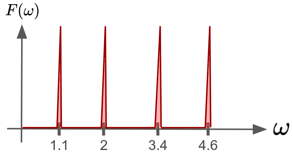
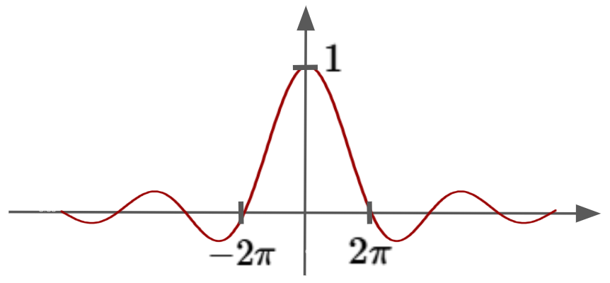
So, with this graph, it’s easy to see what sinusoids make up our original input signal. But what if we have a less obvious square wave as our input $f(t)$?

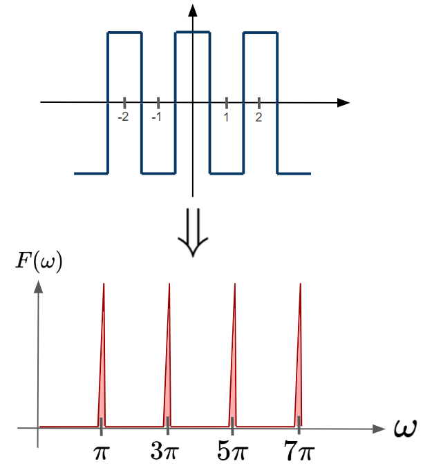
The above $F(\omega)$ graph tells us that the square wave can be represented as an infinite sum of sinusoids (which is the point of the fourier series approximation from the start of this blog!)

$~ \\$

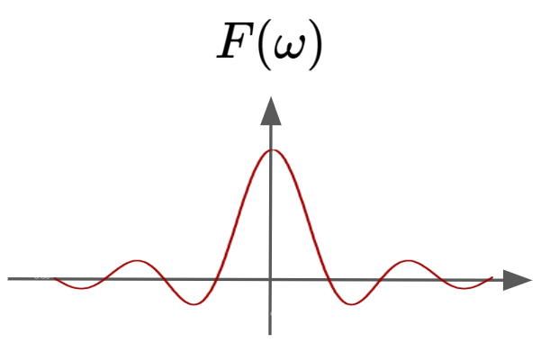
Okay. Now lets find the final piece of this puzzle: we’ve only seen cases of zero and $\infty$ area because we’ve been using periodic functions as our examples. What if we have non-periodic functions with non-zero, finite areas?

Remember this diagram from earlier?

Why is the $F(\omega)$ not “spiky” like in the previous section? Let’s take a closer look:

Let’s say, when doing our computation, we find that:

$\int_{-\infty}^{\infty} f(t) [\cos (3t)] \space dt = 0.66$

Since this is a non-zero value, that tells us that $\cos (3t)$ contributes to the formation of our input square wave like so:

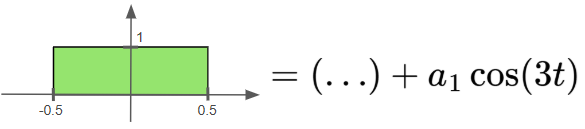
Now, you might be asking, since it’s non-zero, and it contributes to the formation of our square wave, shouldn’t it be an infinite value instead of 0.66? Since, if $f(t)$ is represented as $(\ldots)+a_1 \cos (3t)$, when we do our Fourier Transform and multiply $f(t)$ by $\cos (3t)$, we should get an infinite area under the $\cos (3t)^2$ graph formed.

As it turns out, if $a_1 \rightarrow 0$, we could “approach a finite area”. So, while there is indeed a $\cos (3t)$ term making up our input signal $f(t)$, it is made infinitely small because of $a_1$.

In this example, if we were to check with $\omega = 3.1$, our area is $0.65$. This means $f(t) = (\ldots)+a_1 \cos (3t) + a_2\cos (3.1t)$, but $a_2 \rightarrow 0$ also. This is pretty much the case for every real $\omega$ here.

So, we have to sum up a continuous spectrum of infinitely small sinusoids to produce the rectangular function. Thus, instead of the ‘spiky’ $F(\omega)$ graph mentioned earlier, we have a smooth one like this:

$~ \\$

So, in summary, our Fourier Transform scans for sinusoids that make up our input signal. Now we intuitively know how it does that!

Thank you for reading!

References

1. Dr.Trefor Bazett’s Youtube videos on the Fourier Series
2. These superbly written chapters on the Fourier Series + Transforms by HELM
3. Zach Star’s Youtube video on building an intuition for the Fourier Transform