An Intuition of Singular Value Decomposition

Singular Value Decomposition is one of the most powerful tools in numerical analysis. It generalizes eigenvalue decomposition to any matrix and provides insight into the structure of the matrix, enabling crucial tasks like dimensionality reduction and noise reduction.

It states that:

$\fcolorbox{orange}{white}{$A = UΣV^T$} \\ ~ \\ \space A \in R^{M \times N}, \space U \in R^{M \times M}, \space \Sigma \in R^{M \times N}, \space V^T \in R^{N \times N} \\ \text{U is an orthogonal matrix whose columns are left singular vectors of A} \\ \text{Σ is a diagonal matrix with +ve entries called the singular values of A} \\ V^T \text{ is the transpose of an orthogonal matrix whose columns are right singular vectors of A}$

$~ \\$

SVD has no restrictions on the symmetry, dimensionality or rank of the input matrix.

In this blog post, I will attempt to construct an informal geometric intuition for how SVD works, and why it is so powerful in decomposing matrices.

We’ll begin this blog post by answering some fundamental questions, and gradually build up to SVD.

1. Visualizing rectangular matrices

What’s the difference between a matrix in $R^2$: $\begin{bmatrix} 1, \ 2\end{bmatrix}$ and a matrix with the same entries but in $R^3$: $\begin{bmatrix} 1, \ 2, \ 0 \end{bmatrix}$ ?

Well, the two vectors might have very similar entries, but they exist in different dimensions. Is there a way to transform one to the other?

That’s where rectangular matrices come in - they have the ability to transform the dimensionality of matrices.

A matrix of size $M \times N$ has the ability to transform a matrix from the $M$th dimension to the $N$th dimension. That’s why we say matrices apply a linear transformation from $R^n$ to $R^m$.

$~ \\$

We need to gain a visual understanding of rectangular matrices. Rectangular matrix transformations get visually complicated very easily. So, we’ll begin with two simple cases of rectangular matrices:

1. Dimension Eraser

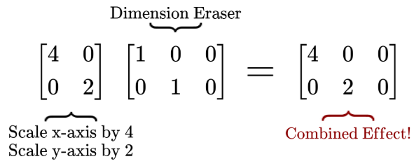
Let’s define a special rectangular matrix below, which we will call the ‘Dimension Eraser’:

$\begin{bmatrix} 1 & 0 & 0 \\ 0 & 1 & 0 \end{bmatrix}$

It looks like an identity matrix with a column of $0$’s on the right side.

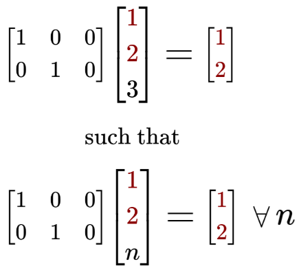
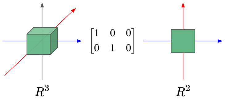
It represents the simplest form of linear transformation from $R^3$ to $R^2$. This is because multiplying the Dimension Eraser with an $\begin{bmatrix} x, \ y, \ z \end{bmatrix}$ vector preserves the $x$ and $y$ component, but ‘erases’ the $z$ component.

Here’s the ‘Dimension Eraser’ in action:

$~ \\$

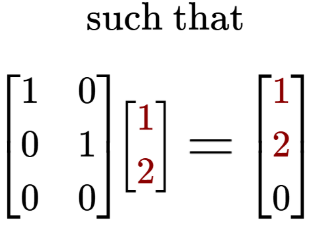
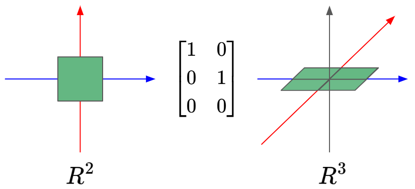
2. Dimension Adder

We can also have the a rectangular matrix that adds dimensionality. In this case we can define the ‘Dimension Adder’ to transform an input from $R^2$ to $R^3$, by adding a zero as the $z$ value to any $R^2$ vector:

$\begin{bmatrix} 1 & 0 \\ 0 & 1 \\ 0 & 0 \end{bmatrix}$

$~ \\$

Combined effects of matrix-matrix multiplication

To end off this chapter, I’d also like to make a quick note about how matrix-matrix multiplication can combine the linear transformation effects of each matrix. For example:

2. Creating a Symmetric Matrix

Recall that a special property of a symmetric matrix is that its eigenvectors are orthogonal to each other.

If we normalize the eigenvectors and package them column-wise into a matrix, we would then have an orthonormal matrix which does a transformation from the standard basis to the eigen basis.

The transpose of the above orthonormal matrix would do the opposite, whereby it produces a transformation from the eigen basis to the standard basis. (If this is not very clear, please read the blog post on Spectral Decomposition)

Most matrices in nature are non-symmetric, which limits the versatility of this eigen basis transformation. Thankfully, we have a way to ‘artificially construct symmetry’!

For a non-symmetric matrix, let’s call it $A$, such that:

$A = \begin{bmatrix} 1 & 2 & 3 \\ 4 & 5 & 6 \\ \end{bmatrix}$

If we multiply $A$ with its transpose $A^T$, we get $AA^T$, which is a symmetric matrix!

$A A^T = \begin{bmatrix} 1 & 2 & 3 \\ 4 & 5 & 6 \end{bmatrix} \begin{bmatrix} 1 & 4 \\ 2 & 5 \\ 3 & 6 \end{bmatrix} = \begin{bmatrix} 14 & 32 \\ 32 & 77 \end{bmatrix}$

Also, if we do $A^T A$ instead, we also get back a symmetric matrix!

$A^T A = \begin{bmatrix} 1 & 4 \\ 2 & 5 \\ 3 & 6 \end{bmatrix} \begin{bmatrix} 1 & 2 & 3 \\ 4 & 5 & 6 \end{bmatrix} = \begin{bmatrix} 17 & 22 & 27 \\ 22 & 29 & 36 \\ 27 & 36 & 45 \end{bmatrix}$

$~ \\$

We should take a moment to appreciate how we just created two different symmetric matrices from a single rectangular matrix $A$. In general, this is true for any matrix $A$.

Here’s a quick proof of the symmetry of $AA^T$, arising from the fact that it is its own transpose: $(AA^T)^T = (A^T)^T A^T = AA^T$.

Next, we’ll see how $AA^T$ and $A^TA$ can be used in finding singular vectors and values.

Singular Vectors and Singular Values

Let’s keep with the example of $A$ being a $2 \times 3$ matrix.

$A = \begin{bmatrix} 1 & 2 & 3 \\ 4 & 5 & 6 \\ \end{bmatrix}$

Now, let’s give our two symmetric matrices some labels:

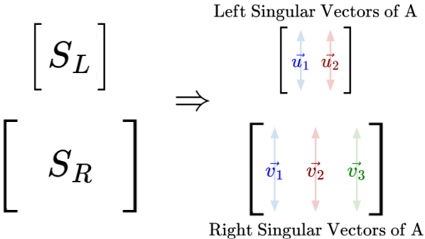
Let’s call our $2 \times 2$ matrix $AA^T$ as $S_L$, where ‘S’ stands for Symmetric and ‘L’ stands for Left. Then, we’ll call our $3 \times 3$ matrix $A^TA$ as $S_R$, where ‘R’ stands for Right.

Since they are symmetric matrices, we know that they have orthogonal eigenvectors.

So, we know that $S_L$ would have two perpendicular eigenvectors in $R^2$, and $S_R$ would have three perpendicular eigenvectors in $R^3$.

Since those eigenvectors are closely related to the original matrix $A$, we’ll call the eigenvectors of $S_L$ as the Left Singular Vectors of A. And of course, the eigenvectors of $S_R$ are known as the Right Singular Vectors of A.

$~ \\$

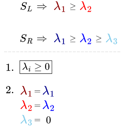
Next, we’ll state two facts without too much side-tracked explanation:

1. $S_L$ and $S_R$ are Positive Semi-Definite Matrices, which means they have non-negative eigenvalues only: $\lambda_i ≥ 0$.
2. When arranged in the same descending order, each corresponding eigenvalue from $S_L$ and $S_R$ have the same value, such that $S_L \space \lambda_i = S_R \space \lambda_i$. Any leftover eigenvalues are guaranteed to be zero.

Just like the singular vectors, these shared eigenvalues are indirectly derived from the original matrix $A$.

If we take the square root of the eigenvalues, such that $\sqrt{\lambda_i} = \sigma_i$, let’s call these square-rooted eigenvalues the Singular Values of A.

The reason why we take the square roots of the eigenvalues to get our singular values can be seen as a way of reversing the squaring effect of $AA^T$ or $A^TA$. For example, the eigenvalues of $A^TA$ represent ‘variances’ along the principal components of data represented by A. So, our singular values (the square root of the eigenvalues) represent the ‘spread’ along the principal component.

Singular Value Decomposition

Now, we’re ready to learn about SVD. Here’s the definition:

$\fcolorbox{orange}{white}{$A = UΣV^T$} \\ ~ \\ \space A \in R^{M \times N}, \space U \in R^{M \times M}, \space \Sigma \in R^{M \times N}, \space V^T \in R^{N \times N} \\ \text{U is an orthogonal matrix whose columns are left singular vectors of A} \\ \text{Σ is a diagonal matrix with +ve entries called the singular values of A} \\ V^T \text{ is the transpose of an orthogonal matrix whose columns are right singular vectors of A}$

$~ \\$

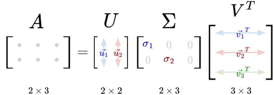
So, SVD tells us that any matrix $A$ can be unconditionally decomposed into three simple matrices, such that $A = UΣV^T$.

Let’s analyze each component more closely:

1. The matrix $\Sigma$ has the same dimensions as matrix $A$, whereby the diagonal entries of $\Sigma$ are the singular values of matrix $A$, arranged in descending order. Every other entry is zero.

2. The matrix $U$ contains the normalized left singular eigenvectors of A, from $S_L = AA^T$, arranged in descending order of the eigenvalues.

3. The matrix $V$ contains the normalized right singular eigenvectors of A, from $S_R = A^T A$, arranged in descending order of the eigenvalues. Then, it is transposed to obtain matrix $V^T$.

Remember, this generalizes to all types of input matrix $A$!

Visualizing the effects of each SVD component

Now, let’s try to visualize the linear transformation effect of each decomposition product. Recall that the resultant linear transformation from an input matrix $A$ is the sequential composition of each decomposition product, $UΣV^T$.

Let’s say we have a matrix $A$, such that:

$A = \begin{bmatrix} 3 & 2 & 2 \\ 2 & 3 & -2 \\ \end{bmatrix}$

and upon doing SVD, we get:

$A = \begin{bmatrix} 3 & 2 & 2 \\ 2 & 3 & -2 \\ \end{bmatrix} = \begin{bmatrix} \frac{1}{\sqrt{2}} & \frac{-1}{\sqrt{2}} \\ \frac{1}{\sqrt{2}} & \frac{1}{\sqrt{2}} \end{bmatrix} \begin{bmatrix} 5 & 0 & 0 \\ 0 & 3 & 0 \end{bmatrix} \begin{bmatrix} \frac{1}{\sqrt{2}} & \frac{1}{\sqrt{2}} & 0 \\ \frac{-1}{\sqrt{18}} & \frac{1}{\sqrt{18}} & \frac{-4}{\sqrt{18}} \\ \frac{2}{3} & \frac{-2}{3} & \frac{-1}{3} \end{bmatrix}$

$~ \\$

Let’s run through the linear transformation effect of each decomposition product, and see how they compose together:

$~ \\$

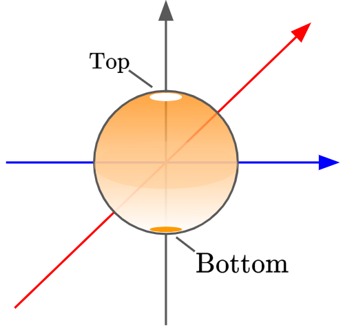
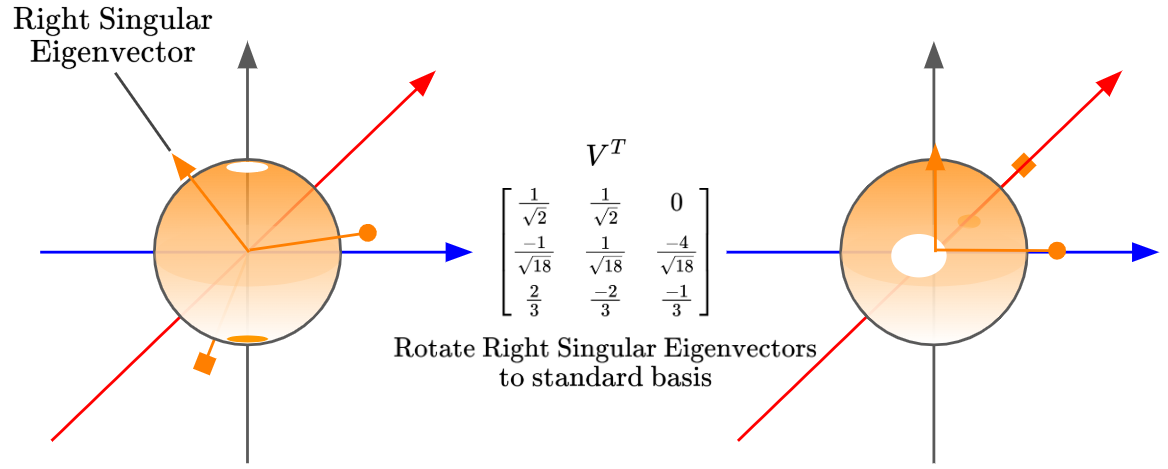
Firstly, we have our input region, and now we’ll go through the linear transformation from matrix $V^T$, which maps our standard basis into the right singular eigenbasis. In easier terms, it ‘rotates’ the right singular eigenvectors to align with our standard basis:

$~ \\$

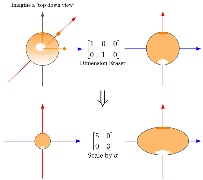
Next, let’s break down the matrix $\Sigma$:

$\begin{bmatrix} 5 & 0 & 0 \\ 0 & 3 & 0 \end{bmatrix} = \begin{bmatrix} 5 & 0 \\ 0 & 3 \end{bmatrix} \begin{bmatrix} 1 & 0 & 0 \\ 0 & 1 & 0 \end{bmatrix}$

So, we can see that the matrix $\Sigma$ actually has two linear transformation effects: firstly, the Dimension Eraser, then a scaling of the $x$-axis by a factor of 5, and the $y$-axis by a factor of 3. These scaling factors are given by our singular values, $\sigma$.

$~ \\$

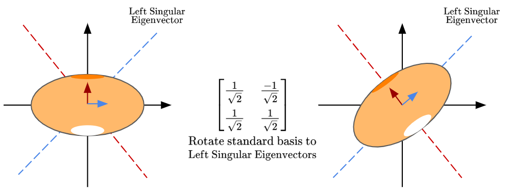
Finally, the matrix $U$ preserves the geometry of the ellipse formed, but rotates the standard basis to align with the left singular eigenvectors:

So, in summary, by using SVD, we’ve visualized the complicated linear transformation effect of our matrix $A$, by breaking it down into simpler matrices which represent simpler linear transformations, like change of basis, ‘dimension eraser’ and scaling.

An alternate interpretation of SVD

What was demonstrated above is not the only interpretation of SVD.

SVD can also be interpreted as a sum of rank-1 matrices:

$A = U \Sigma V^t \\ \space \\ \Downarrow \\ \space \\ A = \displaystyle\sum_{i=1}^r \sigma_i u_i v_i^T$

$~ \\$

Whereby:

$~ \\$

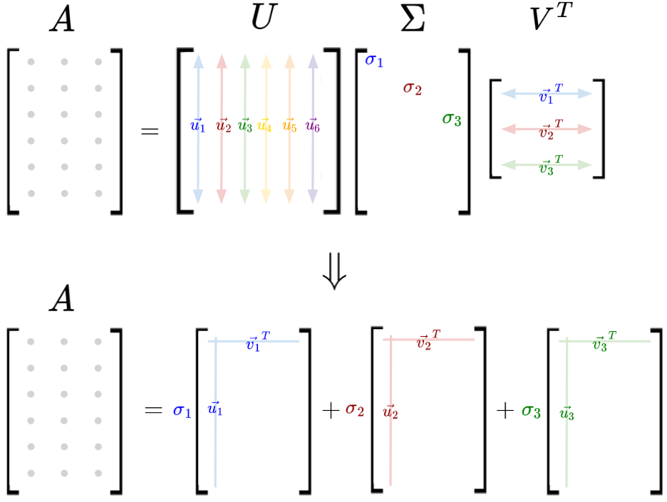
One popular use for this interpretation is in image compression. Let’s imagine our matrix $A$ to have entries that represent pixel properties (let’s say, intensity) in an image. Then, we can interpret the image like so:

$~ \\$

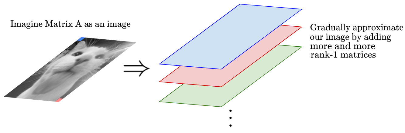
Here’s the logic for why we can approximate an image with this interpretation, and how this can be used for image compression:

1. A rank-1 matrix is a matrix with exactly one linearly independent row and one linearly independent column. So, all of its columns/rows are scalar multiples of each other.

2. This rank-1 matrix spans only a single direction in the ‘matrix space’.

3. Therefore, $\sigma_i u_i v_t^T$ is a matrix that stretches the rank-1 contribution in a direction specified by $u_i$ in the row space and $v_i$ in the column space, by a factor of $\sigma_i$.

4. The largest singular values correspond to the most significant directions in which $A$ acts, so rank-1 matrices with larger singular values $\sigma_i$ dominate the structure of $A$ (or, are most influential in constructing the structure of $A$).

5. By truncating SVD to only include the largest $k$ singular values, we can approximate $A$ as the sum of the most important $K$ rank-1 matrices. This is the basis for low rank approximation (or, image compression). Also, small singular values often represent noise, so there might be noise reduction as well!

$~ \\$

SVD is a beautiful tool, and it’s considered one of the strongest highlights of a linear algebra education. As we’ve seen, it has many wonderful properties that make it a formidable analytical tool. Thank you for reading!

References

This blog post was entirely based on Visual Kernel’s excellent video on SVD!