Gaussian Copula Models
I attempt to explain the concept of Gaussian Copulas as simply as possible.
One evening, when doing some literature review of synthetic data generation methods, I stumbled upon a paper that used Gaussian Copula models for understanding correlations between particular columns.
This blog post is a record of my attempt to understand Gaussian Copulas in an evening. It won’t be the most mathematically in-depth, but hopefully it is helpful in building some basic intuition!
Introduction to Gaussian Copula
Gaussian Copula are widely used in various fields due to their ability to model and simulate dependencies between random variables. In my use case, Gaussian Copulas are used for generating synthetic data while preserving correlations in multivariate datasets.
They are so powerful because they allow for separate modeling of marginal distributions and variable dependencies, which allows them to model multivariate scenarios. They are also considered computationally efficient!
Here’s a simplified way to understand how it models relationships between variables:
Let’s say we have two variables, $U_1$ and $U_2$. They are variables with distribution functions which might be different from each other. But we know that these two are correlated somehow. Then, we decide it is safe to assume that the relationship between these two variables can be captured using a (multivariate) gaussian-type distribution. Since in this example, we have two variables, we thus have a ‘2D Gaussian Copula’ that describes the relationship between our two variables. Below, we visualize the density plot of our Gaussian Copula in an interactive plot.
Okay, now we have some basic technical ideas about why gaussian copulas are used:
- We have a few random variables, which have possibly different distribution functions
- We don’t exactly know how they might be related to each other, but we do know they are correlated somehow
- We decide to model their dependence on each other by a multivariate-gaussian distribution
- And, we describe their level of dependence/correlation by finding the correlation matrix
- Then, we can see how changes in one variable can affect the other(s)!
Next, we will specify in more detail what Copulas are.
What exactly are Copulas?
When learning a new concept, I like to do some reading on why that concept is named the way it is. The word ‘Copula’ means to ‘tie’ or ‘bond’, and it is actually the root word for ‘couple’. So, Copulas allow us to couple the individual distribution functions of each variable together and specify their correlation separately. The Copula therefore is a coupling function that outputs a joint probability distribution.
Next, to learn more about how Copulas work, we need to understand how Cumulative Distribution Functions and Probability Integral Transforms work first.
Cumulative Distribution Functions
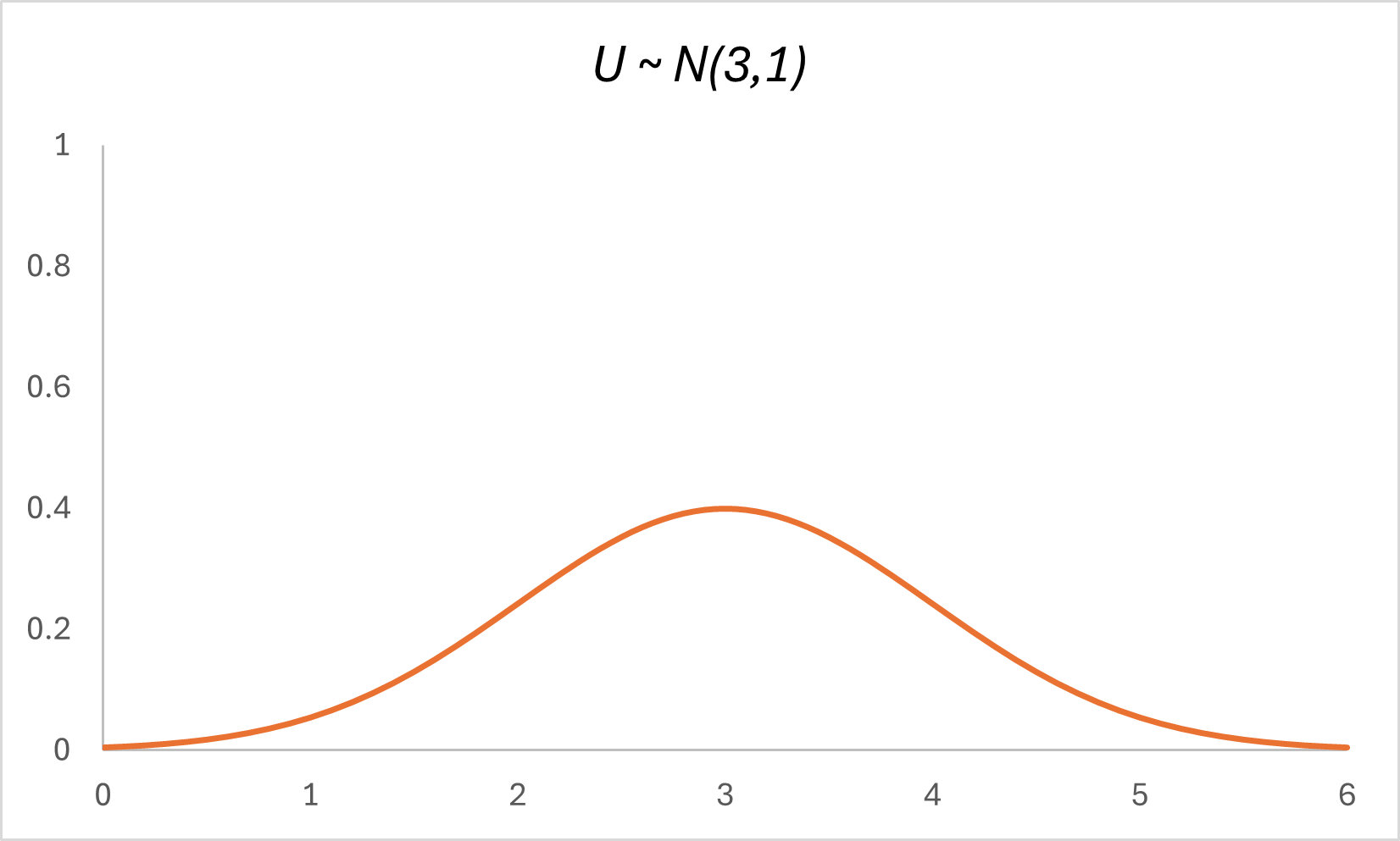
So let’s say we have a random variable $U$ that is normally distributed, with its mean about $x=3$ and standard deviation of $1$, such that $U \space \sim \space N(3,1)$. Here’s the Probability Distribution Function of $U$:
The Cumulative Distribution Function of $U$ is defined as:
Whereby the right-hand side represents the probability that random variable $U$ takes on a value less than or equal to $x$.
In simple words, $F_U(x)$ has a value that keeps increasing, from $0$ to $1$. When $F_U(x) = 0.8$, $x$ represents the $80$th percentile of the distribution of $U$.
Here’s what the CDF plot for our random variable $U$ would look like:
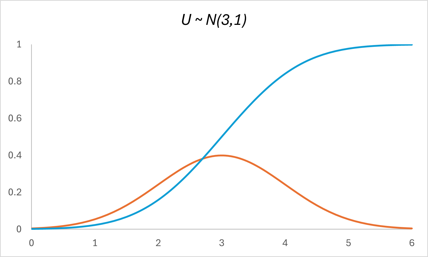
The CDF looks so drastically different from the normal distribution. Let’s analyze why: observe that the region of steepest gradient on the CDF coincides with the mean of the normal, while the regions of weakest gradient on the CDF align with the tails of the normal.
This happens because normal distributions have a high probability density near their mean and lower densities in their tails. As $x$ increases along the horizontal axis, the cumulative probability (represented by the CDF) increases more rapidly in the region around the mean, where the PDF is high. Conversely, in the tail regions, where the PDF is lower, the cumulative probability increases more slowly.
Now, we’re ready to learn about the Probability Integral Transform, or the ‘Universality of the Uniform’.
Probability Integral Transform
The Probability Integral Transform sounds intimidating, but it can be described by a (somewhat) simple statement:
Suppose that a random variable $U$ has a continuous distribution, whereby its Cumulative Distribution Function is $F_U$. Then, if you have a random variable $Y$ whereby $Y \space := \space F_U(U)$, the random variable $Y$ has a standard uniform distribution.
Okay, so, let’s say my random variable $U$ is normally distributed, and if I plot the values of my random variable $U$ back into its CDF, I get back a random variable $Y$ that is unformly distributed.
Let’s try to visualize this:
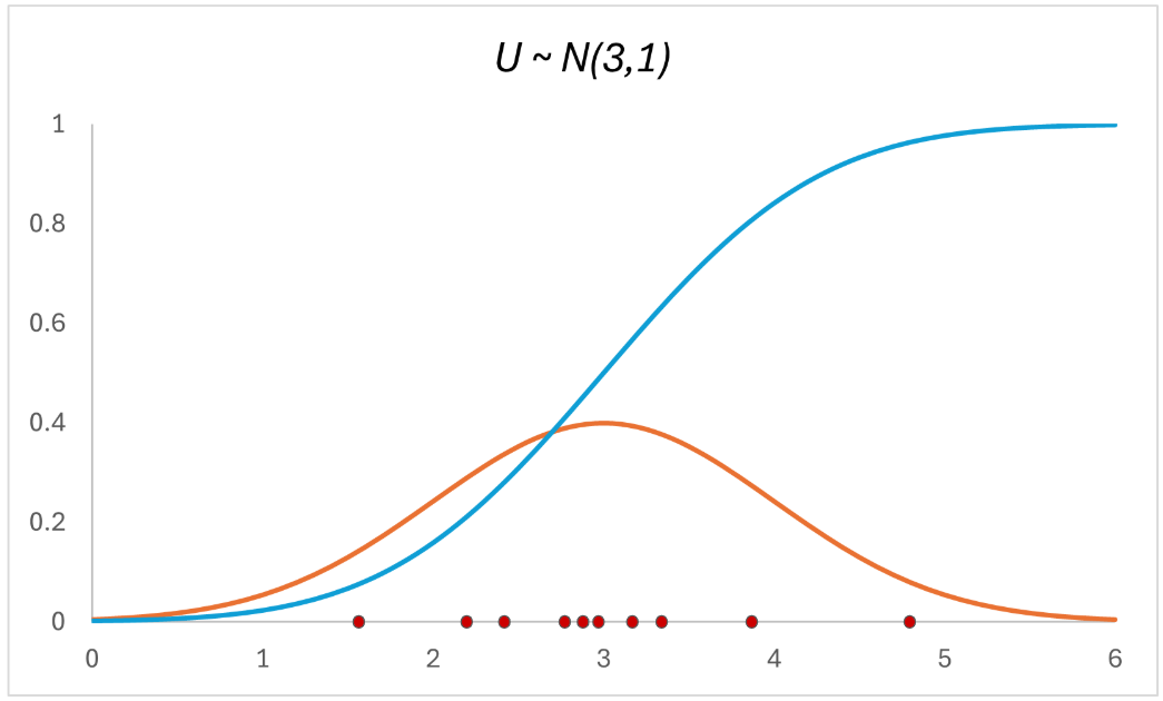
Firstly, we’re going to randomly sample 10 data points of our normally distributed variable $U$. We can see them in the red dots on the horizontal axis:
Next, like the Probability Integral Transform says, we’re going to plug these data points of $U$ back into its CDF, such that we get $F_U(U)$:
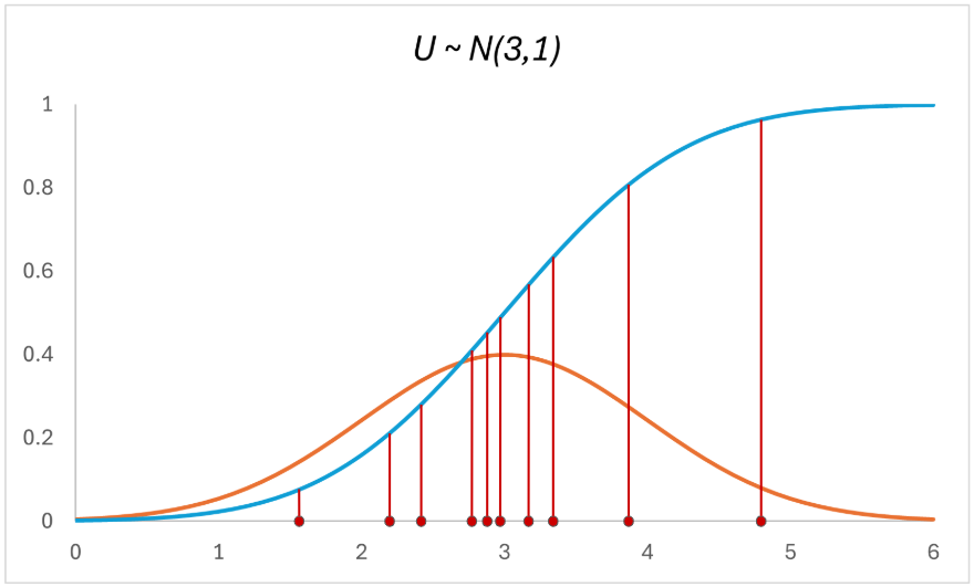
And we’re going to get back the 10 points on the vertical axis:
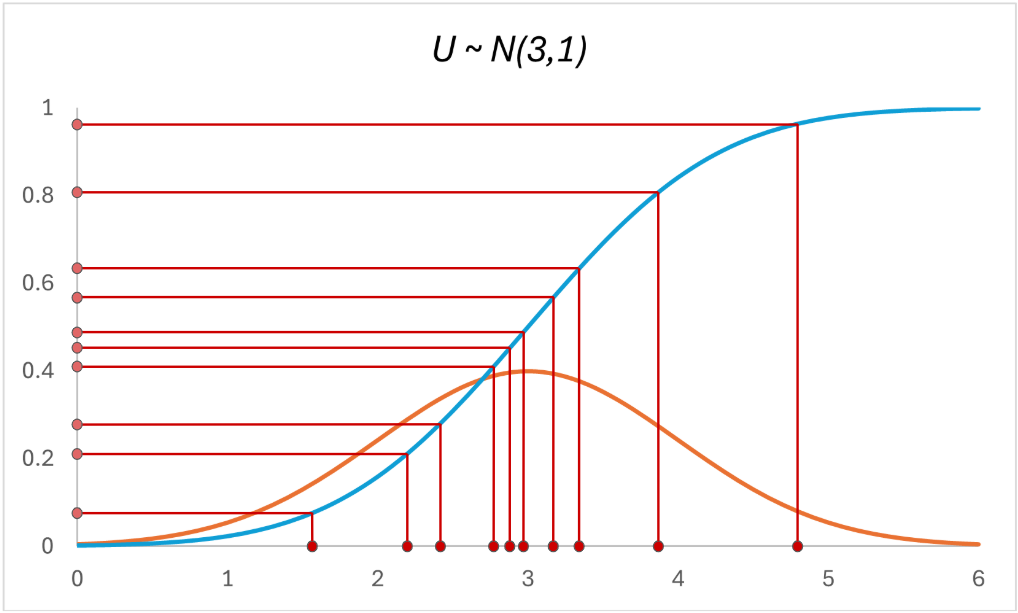
To understand the Probability Integral Transform, we need to see the CDF as a probability mapping, whereby $F_U(U)$ maps every value of $U$ to its cumulative probability.
Notice that the distribution of the 10 points on the horizontal axis looks different from that of the 10 points on the vertical axis? The vertical samples look a lot more uniformly distributed than the horizontal samples (which are normally distributed).
This is because of the changing slope of the CDF. When we apply the CDF $F_U(U)$ to the samples from the normal distribution, recall that:
- In regions where PDF is high (around the mean), the CDF’s slope is steep because probabilities accumulate faster
- In regions where PDF is low (around the tails), the CDF’s slope is gentler because probabilities accumulate more slowly.
As a result, the concentration of samples in the high-density region of the normal distribution is ‘spread out’ more evenly when mapped through the CDF.
This spreading effect of the CDF exactly counteracts the clustering of the original normal distribution. As a result, regardless of how the variable $U$ is originally distributed, the transformed variable $Y \space = \space F_U(U)$ always follows a uniform distribution on [0,1].
Now, we also intuitively understand why Probability Integral Transforms are also called the ‘Universality of the Uniform’.
So far, we’ve worked with inputting random variable values into its own CDF, to obtain a uniform distribution, such that $F_U(U) = Y$. Notice however, if we wanted to get variable $U$ instead, we could do $U = F_U^{-1}(Y)$. This is called the Inverse CDF function.
The CDF and Inverse CDF thus allows us to jump from distribution to distribution!
Now that we understand Probability Integral Transforms, we’re almost done! We will move on to see how this helps us achieve our Gaussian Copulas.
Using Probability Integral Transforms to obtain Gaussian Copulas
Using what we know about Probability Integral Transforms, we can see how they help us obtain gaussian distributions from our starting distributions:
It is also becoming increasingly clear that thanks to the ‘Universality of the Uniform’, the uniform distribution becomes a ‘lingua franca’ for our distribution transformations!
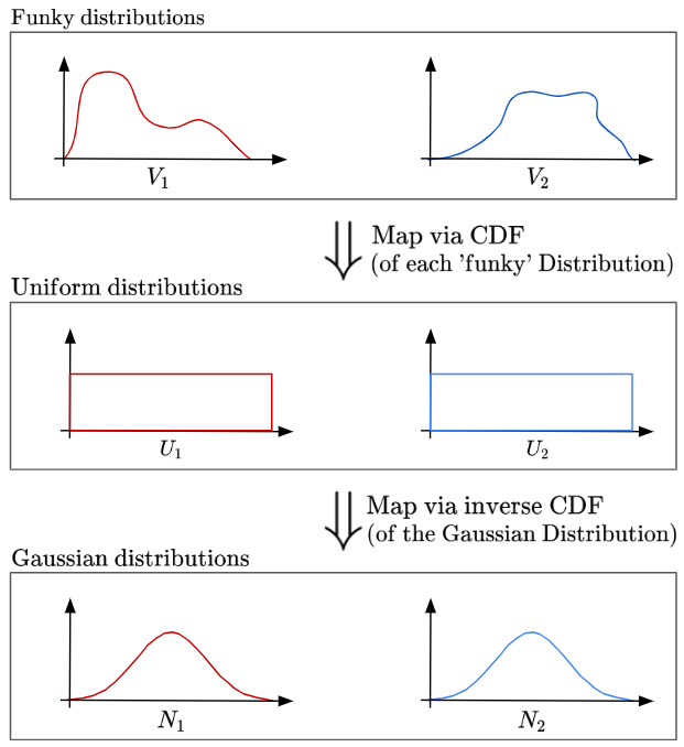
Next, here’s the step-by-step for forming a Gaussian Copula, which we should be able to better understand:
Step 1. Start with random variables $V_1, V_2$ with an arbitrary marginal distribution $F_1, F_2$
Step 2. Apply the PIT to transform $V_1, V_2$ into uniform random variables
Step 3. Apply the inverse of the standard normal CDF (denoted by $Φ^{−1}$) to transform $U_1, U_2$ into standard normal random variables $N_1$ and $N_2$
Step 4. Compute the correlation (or covariance) matrix $Σ$ from the transformed variables in the Gaussian Space
Step 5. Impose the correlation structure (via correlation matrix $Σ$) on $N_1,N_2$ to form a multivariate normal distribution
Step 6. The Gaussian Copula is the joint distribution of ($U_1$, $U_2$) induced by the multivariate normal distribution of $(Z_1, Z_2)$, whereby $Φ_R$ is the joint CDF of the multivariate normal distribution.
In this example, our Gaussian Copula is mathematically defined as:
Perfect! So now we understand how to actually construct a Gaussian Copula.
To finally accomplish my task of generating synthetic data, I would then randomly sample from this multivariate normal distribution, and do the complete reverse-transformation to obtain values in my original Random Variable Distribution (Eg. $V_1$,$V_2$). Thus, we have pseudo-randomly generated data that look similar to our original input random variables.
I hope this short blog post was able to give a decent intuition for how Gaussian Copulas work.
Thanks for reading!
References
- I enjoyed the explanation in this great blog post by Thomas Wiecki
- I also found this short video on the Probability Integral Transform by Brian Zhang particularly intuitive!