Visualizing the Self-Attention Mechanism

In this post, I will attempt to rationalize my geometric intuition for how Self-Attention works in Large Language Models.

Here’s the structure for this writeup:

1. Intuitive Explanation of Attention
1.1 Embeddings & Context
1.2 Similarity
1.3 Attention
1.4 Keys & Queries Matrices
1.5 Values Matrix
1.6 Self Attention
2. References

1. Intuitive Explanation of Attention

In this section, we will go through some intuitive explanations of Attention and its core components. We’ll cover the role of embedding, context and similarity measures, before going deeper into defining Attention, and the K-Q-V components.

$~ \\$

1.1 Embeddings and Context

Let’s begin with an input sentence. We need to represent this sentence mathematically, so that it can work with our various machine learning models.

To do this, we will represent each word (or token) in the sentence as a vector.

As we know, a vector in 3D space might look like [1, 2, 3], representing coordinates along three dimensions. In the context of text, when we embed a word as a vector, we convert it into a similar ordered list of numbers.

Each dimension of the embedding vector represents different aspects of meaning, or relationships between the words.

Embedding vectors are used to capture the semantics of our input text such that similar inputs are close to each other in the embedding space.

Here’s a simple but clarifying example:

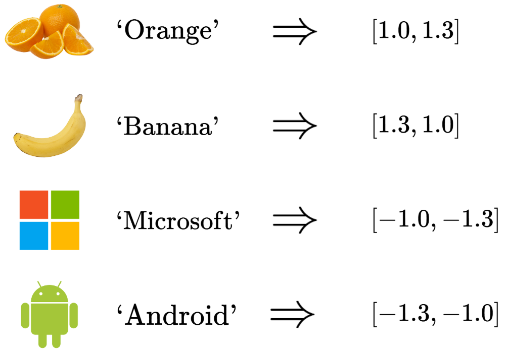
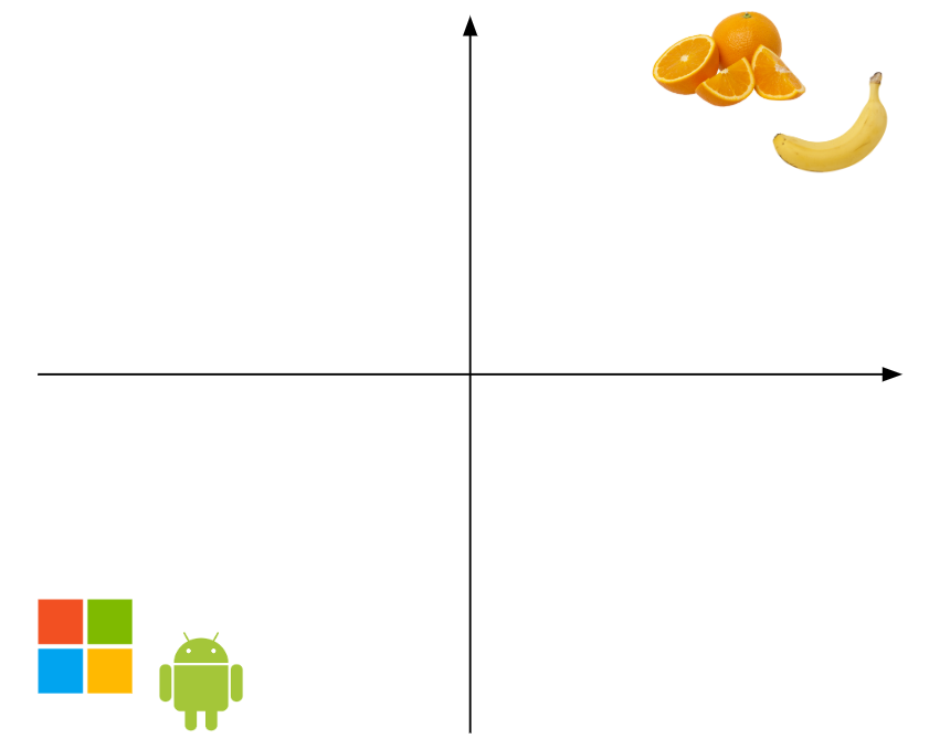
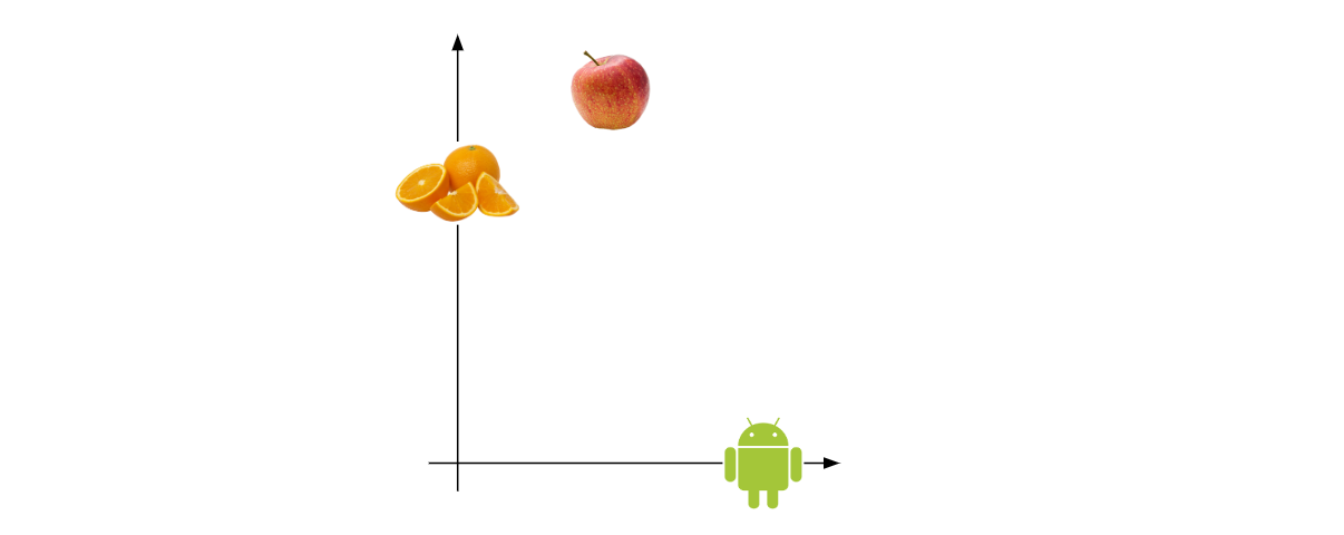
Let’s say we have a bunch of words representing fruits, such as ‘Orange’, ‘Banana’, etc. We also have a bunch of words representing technology products, such as ‘Android’, ‘Microsoft’, etc.

Now, we embed the input words to a 2D embedding space:

$~ \\$

$~ \\$

Now, the question is, where would you put the word ‘Apple’? It could both refer to the fruit, or the tech company.

$~ \\$

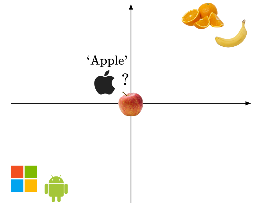
Well, to figure this out, naturally, we would look at the context of the whole input sentence.

For example, given an input sentence ‘Please buy an Apple and an Orange’, then we know for sure ‘Apple’ refers to the fruit. On the other hand, if the sentence was ‘Apple unveiled their new phone’, then we would know that ‘Apple’ refers to the tech company.

Then, we’ll embed the word ‘Apple’ closer to the relevant context-providing word!

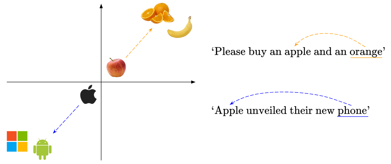
So, each word needs to be given context, which is derived from the neighbouring words. So in the case of the first sentence involving apples and oranges, we’d move the word ‘Apple’ closer to the word ‘Orange’ in the embedding space, where the word ‘Apple’ and ‘Orange’ contribute to each other’s ‘fruit’ context. The mechanism is the same for the second sentence.

In the case of the Attention mechanism, context refers to the information gathered from other words in the sentence, that influences the representation of a given word. To be clear, ‘context’ is not a single variable or metric, but rather an emergent property of how tokens are related and influence each other dynamically based on meaning and position.

$~ \\$

1.2 Similarity

Now, hopefully we see why understanding the context of the input text helps us decide on the best way to represent the relationships between the input words (via their embeddings).

In the earlier example, we saw how the word ‘Apple’ moves closer to ‘Orange’ in the embedding space when our input text refers to fruits. This means that words with similar meanings are represented as vectors that are close together in the embedding space, while unrelated words are farther apart.

Okay, then the next question naturally becomes, how do we know that we’ve embedded our words correctly? Meaning, how do we know when similar words like ‘Apple’ and ‘Orange’ have been correctly embedded to be vectors that lie closer to each other?

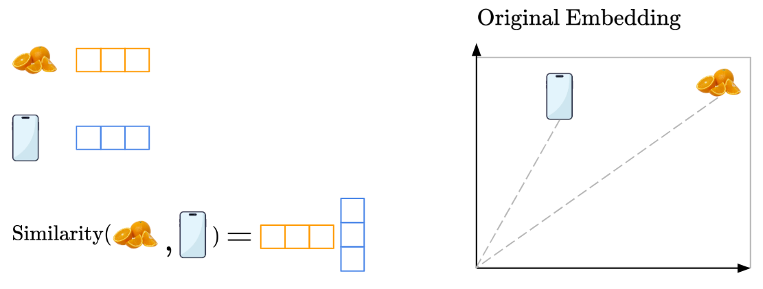
To do that, we’ll need a way to measure the similarity of the embedded vectors!

One common way we measure similarity is by using the Dot Product of the embedding vectors. We’ll illustrate how the Dot Product works:

Firstly, recall that in the embedding space, each dimension represents some relationship or meaning within the input text. For example, given our earlier input words (‘Orange’, ‘Android’, etc.), our 2D embedding space could include one dimension representing the ‘Fruit’ characteristic and one dimension representing the ‘Tech’ characteristic of our input text, like so:

Let’s say we have the following setup:

Then, the dot product computation would be like so:

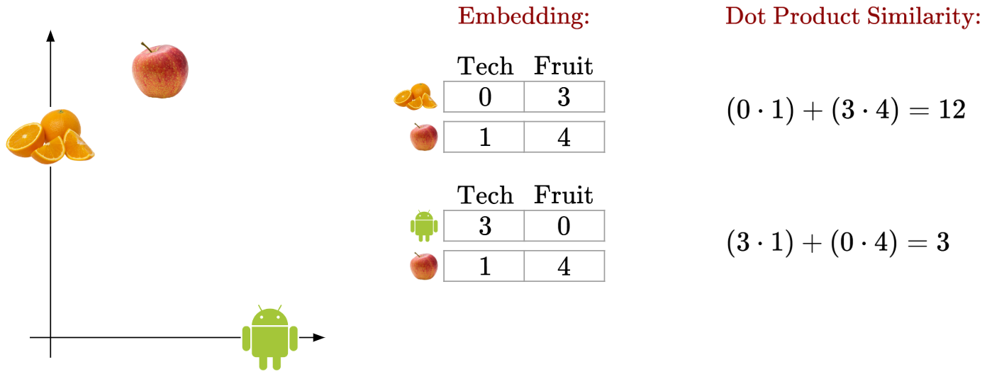
We can see that words that are similar, like ‘Apple’ and ‘Orange’, will have a greater dot product value, while words that are dissimilar will have a smaller dot product value.

Additionally, we can see how the dot product of the ‘Orange’ and ‘Android’ embedding vectors would be 0 (due to their orthogonality). This ensures that words that are purely about fruits and words that are purely about tech have no dot product similarity.

$~ \\$

However, the Dot Product is not a perfect measure of similarity, because it can be influenced by the magnitude of vectors involved.

There are other measures of similarity like Cosine Similarity, but the original Attention Mechanism in the 2017 paper uses something called Scaled Dot Product Similarity. It is simply the Dot Product divided by the square root of the length of the vector.

$~ \\$

Okay, to summarize what we’ve learnt so far:

• We need to embed words as vectors in an embedding space.
• To determine the optimal embedding location for each word, we need to understand the context of each sentence.
• To measure how well we’ve embedded similar words together, we will measure the similarity of their embedding vectors, using tools like the Dot Product, Cosine Similarity, or Scaled Dot Product Similarity.

$~ \\$

1.3 Attention

In this section, we’ll see how to apply the ‘Attention’ step to our token embeddings. Attention represents how much focus we should give to the other words in an input sentence when processing each word in it.

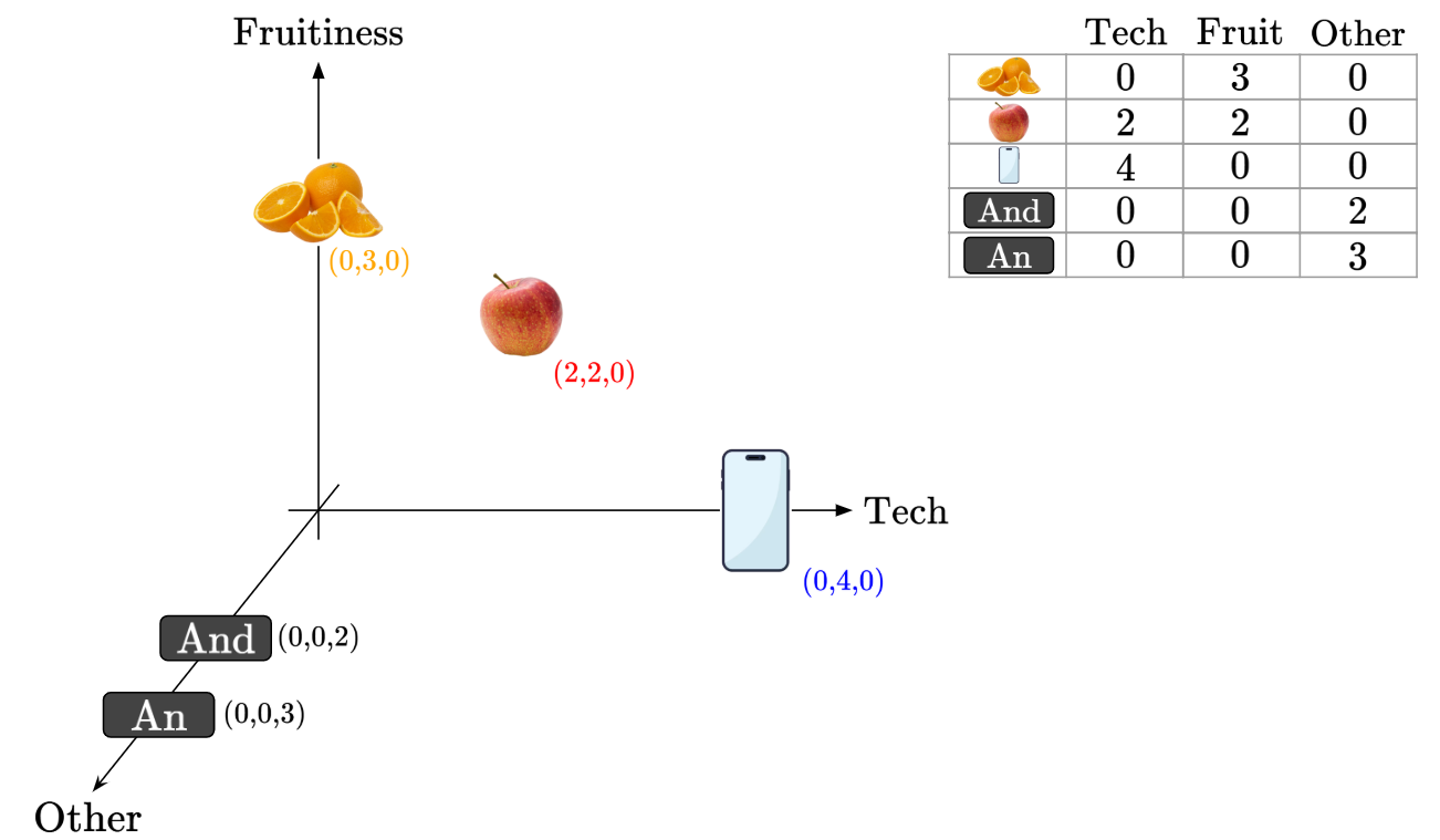
Let’s say we have an 3D embedding for the words ‘Orange’, ‘Apple’ and ‘Phone’, along with grammatical words like ‘And’ and ‘An’, like so:

Let’s find the similarity value between each pair of words (i.e. each pair of embedded vectors). For simplicity of computation, we’ll use Cosine Similarity, but you can imagine that any other similarity measure would work too.

This pairwise similarity measure will help us understand how the existing words in an input sentence will influence each other word.

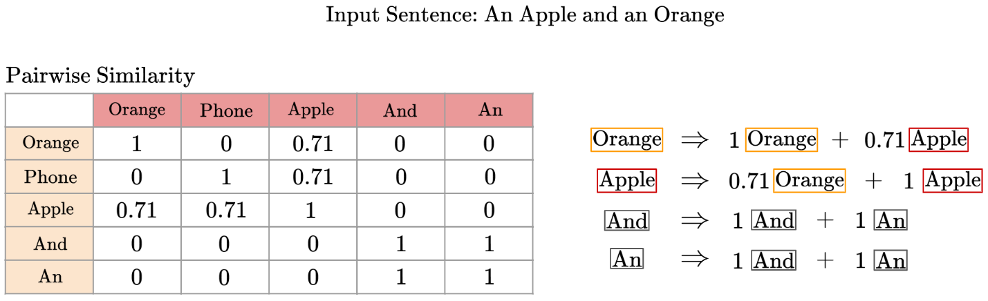
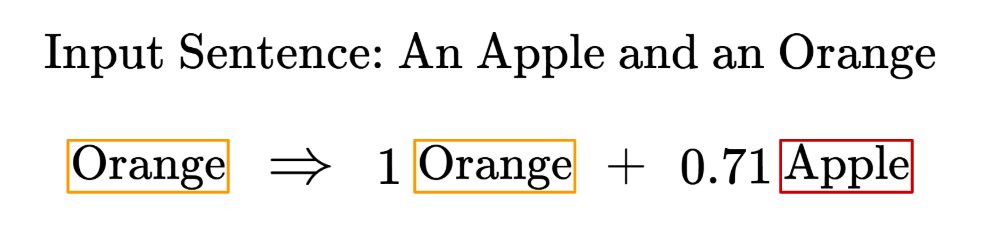
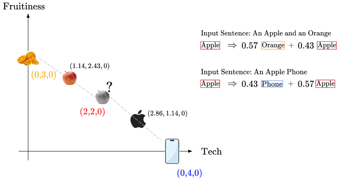
Take for example, given the input sentence ‘An Apple And An Orange’, and the pairwise similarity table:

$~ \\$

Another example - what if our input sentence was ‘An Apple Phone’?

$~ \\$

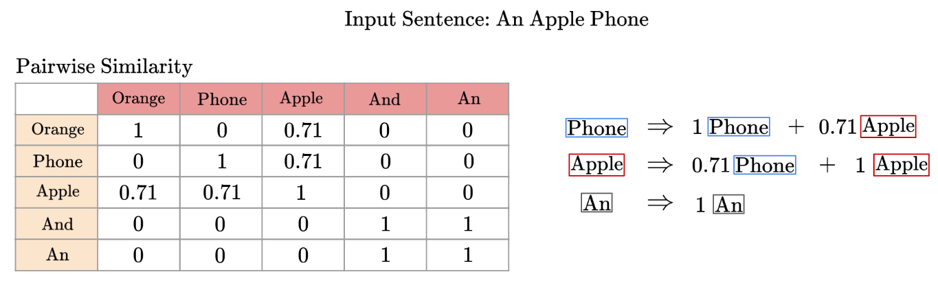
So now, we have a way to mathematically describe how much each other word in an input sentence influences, or provides context to each word:

We’ll want to prevent the magnitude of the coefficients from growing out of control, and handle negative coefficients, so we’ll apply the SoftMax function to these values:

$~ \\$

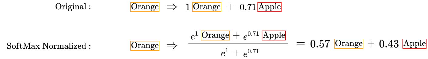
However, just to be a little more mathematically rigorous, we need to take note that the SoftMax function also assigns any 0 value a real positive value now. For example, recall the pairwise similarity score for the word ‘Orange’:

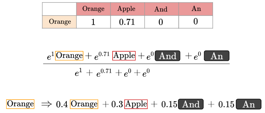
For our example, we’ll simply acknowledge that they hold relatively smaller influence and we’ll ignore these extra terms for simplicity’s sake.

$~ \\$

Let’s go back to our pairwise similarity equations. Given the equations, we can say that after taking into account the original embedding of the word ‘Apple’ and the pairwise similarity values with other words, we will account for the influence of the other words and adjust our embedding.

For example, given the input sentence ‘An Apple And An Orange’, we’ll take 43% of the original ‘Apple’ embedding values and replace it with the ‘Orange’ embedding values instead. Geometrically, this means we’re taking the line between ‘Apple’ and ‘Orange’, and moving it 43% of the way closer:

So, we can see that the embedding of the word ‘Apple’ has improved, after taking into account the context of the other words. We can imagine that for many words, across many rounds of iterations, our embeddings will improve significantly and similar words will be optimally grouped together.

Thus, we can see the benefit of paying ‘Attention’ to the other important context-providing words in a sentence. This is the essence of the attention mechanism.

$~ \\$

1.4 Keys and Queries Matrices

In the previous section, we learnt how applying the ‘Attention step’ (where we compute the pairwise similarity scores and modify our original embedding) allows us to improve the original word embeddings.

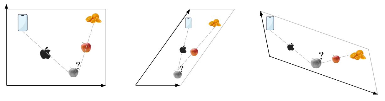
Recall that we have the embedding visualization for the word ‘Apple’, along with ‘Orange’ and ‘Phone’.

What if our embedding was slightly different? Let’s see three examples:

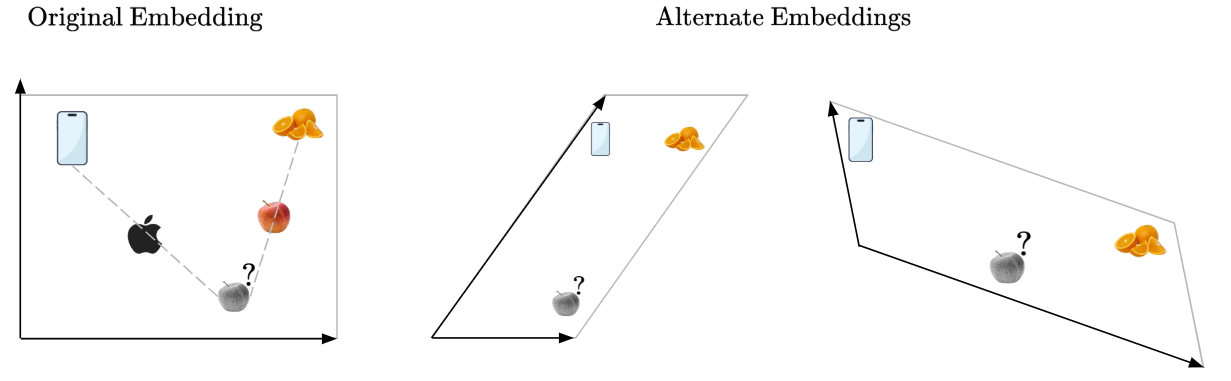
Which embedding space would be the best for applying our ‘Attention’ step to?

We can see that the middle embedding is not ideal, because our ‘Apple’ embeddings will not be very distinctly separated even after calculating the pairwise similarity and applying the ‘Attention’ step. On the other hand, the rightmost embedding is ideal because it makes the separation between our ‘Apple’ embeddings even more distinct:

Hence, the point is clear that some embedding spaces are better than others. Now, how can we attain the rightmost embedding space from our original embedding space?

Recall that matrices represent combinations of linear transformations. Could we use matrices to linearly transform our original embedding space?

Here’s where the Keys and Queries matrices come in.

So, let’s say you have an input sentence containing the words ‘Orange’ and ‘Phone’. As we’ve seen, we need to embed them as vectors in an embedding space.

Now, let’s say we’re trying to figure out how much attention the ‘Orange’ vector should give to the ‘Phone’ vector. In that case, the ‘Orange’ vector is the ‘Query’, while the ‘Phone’ vector is the ‘Key’ (the comparison point used for computing similarity).

Originally, without the Keys and Queries weight matrices, we would directly compute the pairwise similarity of the raw ‘Orange’ and ‘Phone’ vector embeddings and achieve this original embedding space:

However, we now know that this original embedding space may not be optimal for computing attention. Instead, we apply linear transformations via the Keys and Queries weight matrices to project the embeddings into a space where similarity is more meaningful for attention:

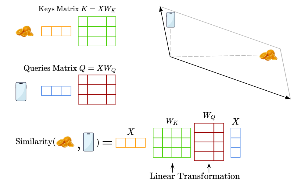
So in summary, the Keys and Queries weight matrices are a way to transform our original embeddings into a more optimal one for calculating pairwise similarities. The resulting matrices containing our linearly transformed token embeddings are called the Keys Matrix and the Queries Matrix.

One might also ask, why do we need both two matrices for the intended linear transformation? Using different learned matrices allows the modelt to optimize the embedding/representation separately for queries and keys. This means the model can optimize what the “queries” are asking for, and what “keys” are offering as information. In effect, using two matrices instead of one allows the model to learn fine-grained attention patterns better.

To summarize our learnings formally, what we’ve found with the Keys (K) and Queries (Q) matrices is:

$\boxed{A = \text{softmax}(\frac{QK^T}{\sqrt{d_k}})}$

Whereby:

• $\text{A}$ is the resulting attention weight matrix, containing values between 0 and 1, representing how much focus/attention each token should give to each other token
• $\text{Q}$ is the Query Matrix, representing the transformed embedding of the queries for each token, where $Q = XW_Q$
• $\text{K}$ is the Key Matrix, representing the transformed embedding of the keys for each token, where $K = XW_K$
• $d_k$ is the dimensionality of each key vector

$~ \\$

1.5 Values Matrix

So we’ve learned that the Keys and Queries matrices help us find the ideal embedding space to find pairwise similarities between our embedding vectors. The resulting computation allows us to find the attention scores of each token - so the Keys and Queries matrices tell us how much focus each token should get.

However, this does not mean that the resultant embedding space from the Keys and Queries transformations is an ideal one for deciding what actual information should be used, or what the best choice is for the next word in the generated output sentence.

Instead, we need another matrix, called the Values weight matrix, to produce a linear transformation, such that we have an optimal embedding space for conveying information. That way, we can obtain the values $V = X W_V$.

Then, we’ll use the Attention Weights obtained from the Keys and Queries matrices to optimize the embedding in our Values matrix embedding space. Let’s see how this works visually:

$~ \\$

$~ \\$

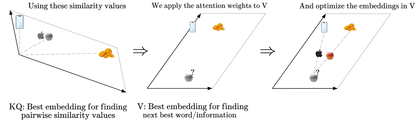
To summarize the learnings from the Values Matrix, we can simply say:

• Value (V) contains the vector embeddings of each token after linear transformation by $W_V$
• Using the attention weights $A$, we find the weighted value embeddings, $AV$
• So if $A$ represents the “Attention Weights” over all words, and $V$ contains the “actual information”, $AV$ gives us a new, context-aware representation of each token.

$~ \\$

Okay, now we have a lot to juggle, so let’s simplify even further and recap on these three matrices and their roles:

• Query (Q) asks: if I am (this) word, who is relevant to me?
• Key (K) answers: if you are (this) word, here’s how relevant each other word is to you
• Value (V) provides: given the computed attention scores, which information should I output next?

$~ \\$

1.6 Self-Attention

Now, let’s quickly formalize what we’ve learnt. The core formula for scaled dot-product self-attention is:

$\boxed{\text{Attention}(K,Q,V) = \text{softmax}(\frac{QK^T}{\sqrt{d_k}})V}$

Visually, the operations that happen within the scaled dot-product self-attention formula are like so:

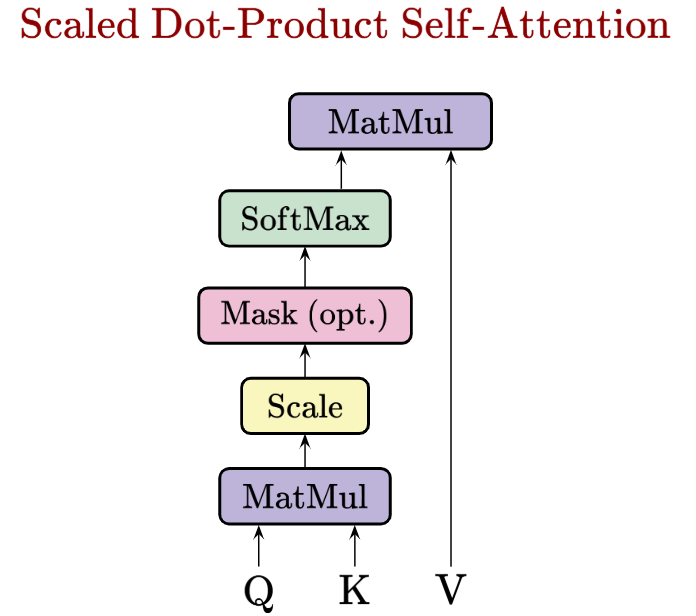
The output of the attention formula is a new set of token embeddings, often called the contextualized representations of our tokens.

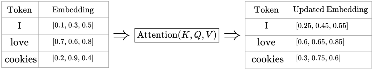
Downstream, this attention output (the contextualized token embeddings) might be passed into a neural network for further refining, then each final token embedding might be mapped into a probability distribution over the entire vocabulary. This allows us to do next-word prediction, and create useful sentences like GPT does.

Okay, perfect! We’re about done with this post. Now, we know how Self-Attention, especially the K,Q,V matrices work together geometrically to produce the magic in Large Language Models.

Thank you so much for your time!

$~ \\$

2. References

This blog post was entirely referenced from Luis Serrano’s video on the math behind self-attention. Personally, I think his videos are a masterclass on the inner workings of many important algorithms, and also on excellent pedagogy!

However, I found myself having trouble rationalizing my learnings from the video into coherent, concise explanations. So, this blog post was really about dedicating some time to concretize the intuition by conveying them through writing.