Transformers are (actually) Kernel Smoothers
I attempt to share some learnings from Tsai et al. (2019) connecting the Attention Mechanism to Nadaraya-Watson Kernel Smoothing (1964).
In this post, I will share some of my learnings about how the Attention Mechanism in Transformers can be exactly re-expressed as the Nadaraya-Watson Kernel Smoothing mechanism.
This mini-essay will be structured as follows:
- Recap on how kernel smoothing works
- Recap on how the attention mechanism works
- Connecting the attention mechanism with kernel smoothing
- Concluding with a more intuitive understanding of attention
- References
A lot of the content is adapted from Tsai et al. (2019), Professor Cosma Shalizi’s writings and Zhu Ruoqing’s notebook - please refer to the bottom of this blog post for the linked references.
Recap on how kernel smoothing works
Let’s begin by understanding what Kernel Functions are, before moving onto understanding how Kernel Smoothing works.
What are Kernel Functions?
Kernel functions are a way of computing the dot product of two vectors $x$ and $y$ in some (possibly very high dimensional) feature space, which is why kernel functions are sometimes called the “generalized dot product”.
Suppose we have a mapping $\phi: \space R^n \rightarrow R^m$ that brings out vectors in $R^n$ to some feature space $R^m$. Then, the dot product of $x$ and $y$ in this space is $\phi (x)^T \phi (y)$.
Mathematically, a kernel is a function $k$ that corresponds to this dot product, such that $k(x,y) = \phi (x)^T \phi (y)$.
Why is this useful? Kernels give us a way to compute dot products in some feature space without needing to know what the feature space is. (More details in the post about the Kernel Trick)
What is Kernel Smoothing?
Let’s learn about the role of kernel smoothing by working through a simple theoretical problem:
Suppose we have a big collection of inputs and outputs to some function, such that we have a bunch of data points like $(x_1, y_1), (x_2, y_2), …, (x_n, y_n)$. Now, given a new input point $x_o$, how would you make a guess at the value of its corresponding output value, $y_o$?
One intuitive way is to reference the point’s nearest neighbour: find the point $x_i$ which is most similar to $x_o$, then report its output value $y_i$. If we wanted to take into account the information from more neighbouring data points, we could reference the $k$-nearest neighbours, where we average $y_i$ from the $k$ points $x_i$ closest to $x_o$.
However, this doesn’t account for the relative closeness between each point $x_i$ to the point $x_o$. Logically, we’d want to give more weight to points which are closer to $x_o$.
In 1964, E. A. Nadaraya and Geoffrey S. Watson independently came up with a similar idea which solves this type of problem:
Suppose we introduce a kernel function $K(u,v)$ which measures how similar $u$ is to $v$. This kernel function has to be non-negative, and should be at maximum value when $u = v$.
Now, what if we use this similarity measure as weights in the average, such that we have:
We divide by the sum of $k$s, such that we can weight the contribution of each $y_i$ from the dataset. This makes the predicted value of $y_o$ a weighted average.
Thus, the Nadaraya-Watson Kernel Smoothing method.
Let’s quickly observe the difference between K-Nearest Neighbours and Kernel Smoothing below. We’ll use a Gaussian Kernel for this example:
import numpy as np
import matplotlib.pyplot as plt
from sklearn.neighbors import KNeighborsRegressor
from sklearn.metrics.pairwise import rbf_kernel

# Data Generation
np.random.seed(42)
x = np.random.uniform(0, 6, 40)
y = 2 * np.sin(x) + np.random.normal(size=40)
testx = np.linspace(0, 6, 500)

# KNN
knn = KNeighborsRegressor(n_neighbors = 10)
knn.fit(x.reshape(-1,1), y)
y_knn = knn.predict(testx.reshape(-1,1))

# Gaussian Kernel Regression
K = rbf_kernel(testx.reshape(-1,1), x.reshape(-1,1), gamma=5.0)
K /= K.sum(axis=1, keepdims=True)
y_kernel = K @ y

# Plot
plt.scatter(x, y, color='dimgrey')
plt.step(testx, y_knn, color='darkorange', lw=2.5, label='KNN')
plt.plot(testx, y_kernel, color='teal', lw=2.5, label='Gaussian Kernel')
plt.title("KNN vs Gaussian Kernel Regression")
plt.legend()
plt.show()
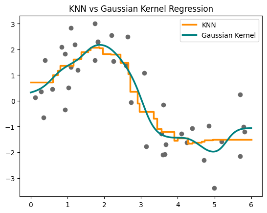
We can see how smooth the kernel plot is compared to the KNN plot.
To end off with some extra details on the kernel function:
Let’s say we have a possible kernel function $K(u,v) = \text{exp} (u \cdot v)$.
Another valid kernel function is $K(u,v) = \text{exp} (w_1 u \cdot w_2 v)$, where $w_1, w_2$ are square matrices.
This is equivalent to $K(u,v) = \text{exp} (u \cdot w_1^T w_2 v)$, which makes it much clearer that we’re actually using the matrix $w_1^T w_2$ to define an inner product between the two input vectors.
Then, to avoid numerical underflow/overflow issues, we normalize by the dimensionality $d$ of the input vectors, such that:
Recap on how the Attention Mechanism works
Recall that the attention mechanism computes a weighted sum of values, where each weight reflects how relevant another input is to a given query.
Given:
- Queries (Q) - what you’re trying to match
- Keys (K) - what you’re comparing against
- Values (V) - the information you’re trying to retrieve
The attention formula is:
Where we first compute the similarity between $Q$ and $K$ via dot product $QK^T$, then scale it by $\sqrt{d_k}$ for numerical stability, then apply softmax to turn the scores into weights, then multiply those weights with the values $V$.
Connecting the attention mechanism with kernel smoothing
Recall that in the attention mechanism, the query, key and value vectors are linear projections of the input embeddings.
For example, given a token at position $q$, its input vector is $x_q = f_q + t_q$, where $f_q$ is the (word) embedding and $t_q$ is the positional embedding.
Then, we compute:
- Query vector $Q$ = $x_q W_q$
- Key vector $K$ = $x_k W_k$
- Value vector $V$ = $x_k W_v$
Whereby each $W_q, W_k, W_v$ is a learned weight matrix, typically shared across all positions in the sequence, and $S_{x(q/k/ v)}$ being the set representation of the query/key/value sequence $x_{ { q/k/v } }$.
Thus, we can rewrite the attention mechanism equation as:
Next, let’s work through a few observations to improve our interpretation of the attention mechanism.
(1) Firstly, we can see that the output is determined by the dot product between $x_q$ and $x_k$ with additional mappings $W_q$, $W_k$, and scaling by $d_k$.
This shows that the dot product, after linear projection and scaling, acts as a learned similarity function, which we can interpret as $K(x_q, x_k)$.
So, the attention uses a learned, scaled kernel like so:
(2) Next, we can focus on the softmax function. We can interpret it as assigning a probability to each key $x_k$, given a query $x_q$, based on how similar they are.
Let’s say you’re given an input sentence: “The cat sat on the mat”. Using self-attention, to find the attention scores for the query “cat”, you’d get the attention distribution: $\text{Pr}( \text{key} | \text{query = “cat”})$.
This provides us with the perspective that the attention mechanism uses “softmax-normalized similarity scores”, which are conditional probabilities.
Then, we can use the probabilities as weights, like so:
(3) Additionally, shown in the equation above, we also introduce a set filtering functon $M(x_q, S_{x_k})$, which returns a set of elements that are visible to $x_q$. Sometimes, not all keys are visible to a query (such as in decoder self-attention, sparse attention, etc), so this function $M(x_q, S_{x_k})$ allows us to define the subset of keys that $x_q$ is allowed to see.
Bringing these together, we can represent the attention equation like so:
We can see that the core structure consists of kernel-weighted average values, and we can see that the attention mechanism is structurally equivalent to Nadaraya-Watson Kernel Smoothing over a filtered subset of keys!
Concluding with a more intuitive understanding of attention
From this perspective, we can understand “Attention” better as a principled statistical operation. When I first learned about the attention mechanism, there was a lot of confusion that arose from thinking of it as a close analogy to human attention, while wrangling with abstract terms like “key”, “query” and “value”.
But by viewing attention through the lens of kernel smoothing, it becomes simple to grasp the concept as a way of computing a weighted average of the values, where the weights are determined by how similar each key is to a given query.
Thank you for reading!
References
This blog post heavily referenced the following sources:
- Tsai et al.’s paper that originally connected the Attention Mechanism to Kernel Smoothing. It’s very readable!
- Professor Cosma Shalizi’s notebook on the same topic. I particularly enjoyed his concise but clear formulation of the use of kernels and their link to the attention mechanism.
- Ruoqing Zhu’s clear writing on Kernels which served as a good recap for me on the topic. The graphics are very helpful!
- This stats.stackexchange post which also served as a good recap on the topic of kernels!