Building Long Short Term Memory (LSTM) from scratch

In this project, I build a LSTM-based model using Pytorch and some math, and we will compare its performance against our previous RNN model in generating sentences.

Published

11 January 2025

In this project, we’re going to build a simple Long Short Term Memory (LSTM)-based recurrent model, using Pytorch.

We’ll employ the LSTM model on the same task as our previous RNN model, and find out which model produces better sentences.

Given the foundational knowledge on RNNs established in previous projects, we’ll move relatively quickly into the theory for LSTMs.

Here’s the structure for this project post:

1. LSTM Overview
2. Forward Propagation
2.1 Backward Propagation
2.2 How LSTMs Solve Vanishing/Exploding Gradients
3. Code Implementation & Results

1. LSTM Overview

In this section, we’ll cover the architecture of the LSTM cell, and examine how it improves upon the basic RNN model we learned in the previous project post. In order to do that, we’ll have a super quick review of RNNs, and modify our visual perspective of RNNs just a little.

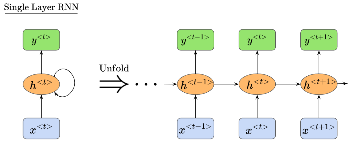
Recall that RNNs are a special type of neural network consisting of recursive computational loops that span adjacent time steps. We visualized them unfolding like this:

Also, recall that our RNN has biases and activation functions. We described the net input to node h as $z_h^{<t>}$, and the activation at node $h$ as $h^{<t>}$, like so:

$\text{Net Input to Node h:}$

$\boxed{z_h^{<t>} = W_{hx} x^{<t>} + W_{hh} h^{<t-1>} + b_h}$

$\text{Activation at Node h:}$

$\boxed{h^{<t>} = \sigma_h (z_h^{<t>})}$

Where the activation function $\sigma_h$ used is usually the $\text{tanh}$ function.

$~ \\$

Now, to prepare for learning about LSTMs, we’ll change our visual understanding of RNNs just a little. Now, we’ll need to see RNNs as forming a chain of repeating modules, with a very simple structure, such as a single $\text{tanh}$ layer:

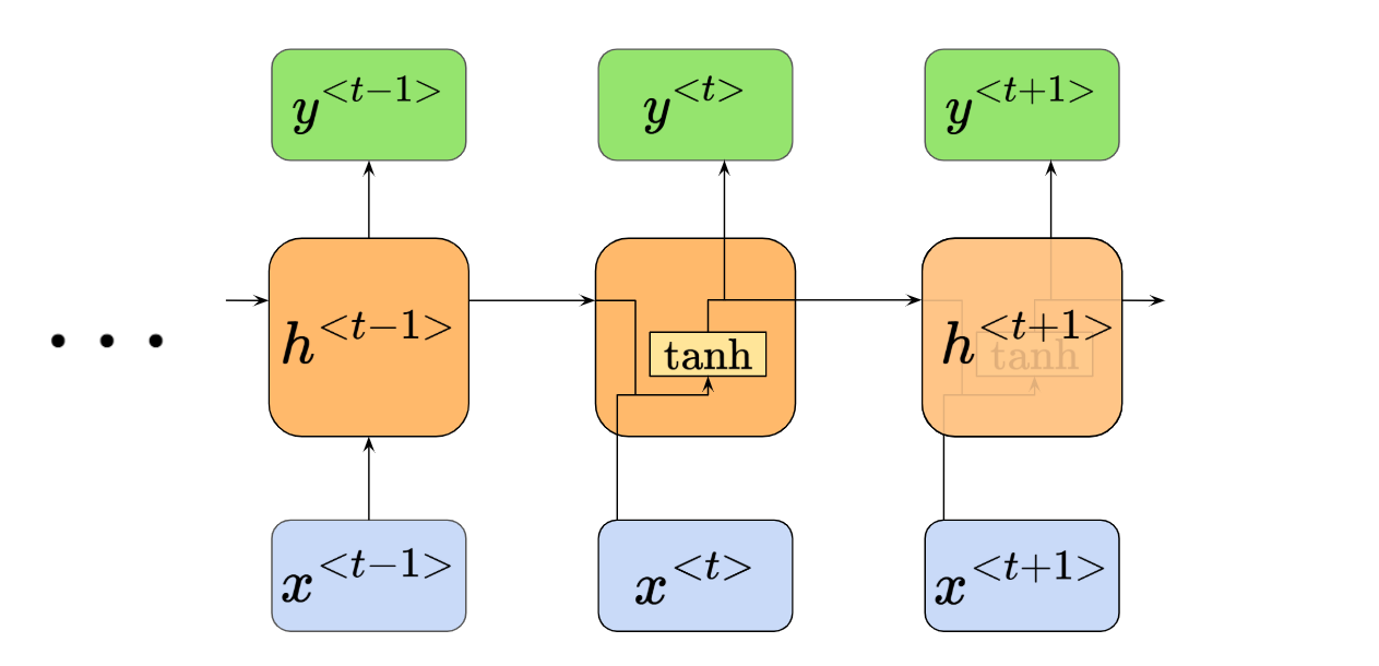
We can see that our node $h^{<t>}$ is now an “x-ray” image of itself, where we can see how the its inputs map to its activation function, and to the outputs. We’ll be using this visual perspective when moving forward to learning about LSTMs next. We’ll also call the central node h as the “repeating module”.

$~ \\$

LSTMs also have this chain-like structure, but the repeating module has a more complicated internal structure. Instead of the single $\text{tanh}$ neural network layer earlier, the LSTM repeating module has four:

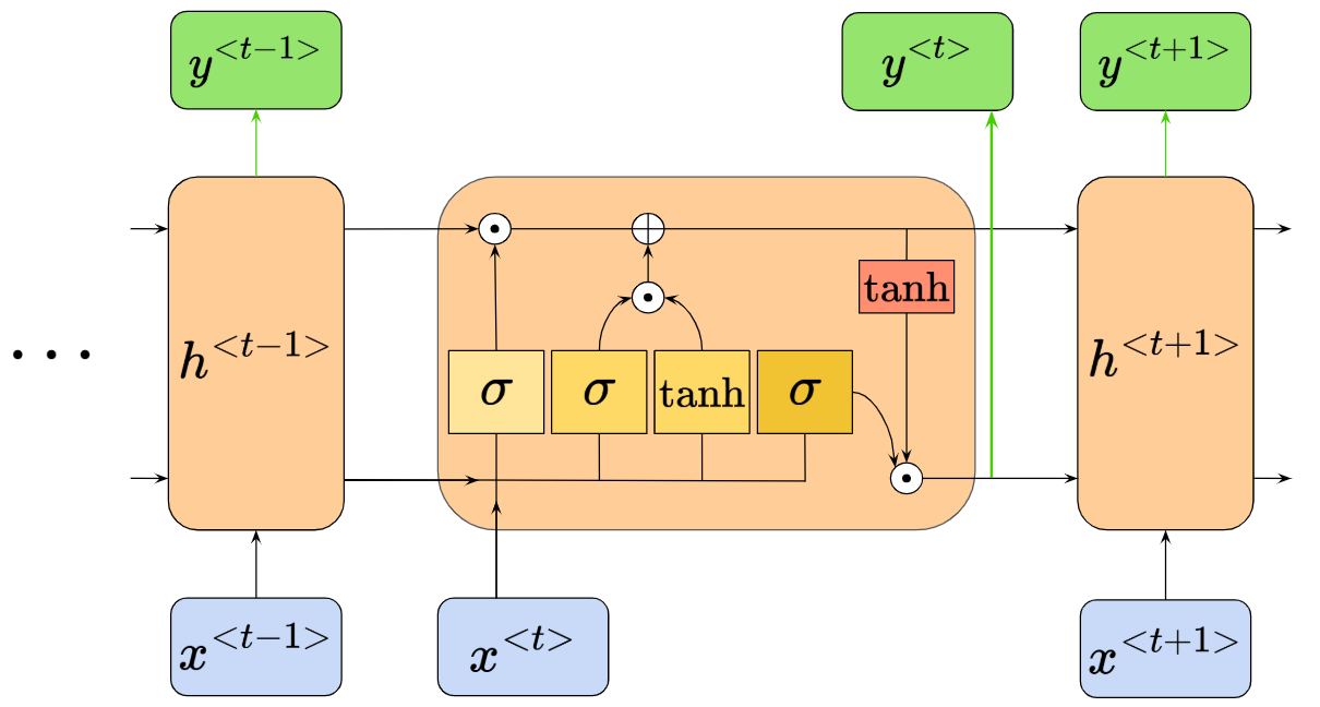
Wow, things got complicated fast. We’ll go into more detail in the next few steps. But for now, the key takeaway is that we now have $\text{tanh}$ and sigmoid $\sigma$ activation functions in our repeating module. There is also also a new input/output at the top of the repeating module, giving us a total of three outputs - two outputs to the next repeating module, one output to node $y$ (colored in green).

$~ \\$

Let’s zoom into a single repeating module for now, and add some labels so we can describe each component. We call this a single LSTM cell:

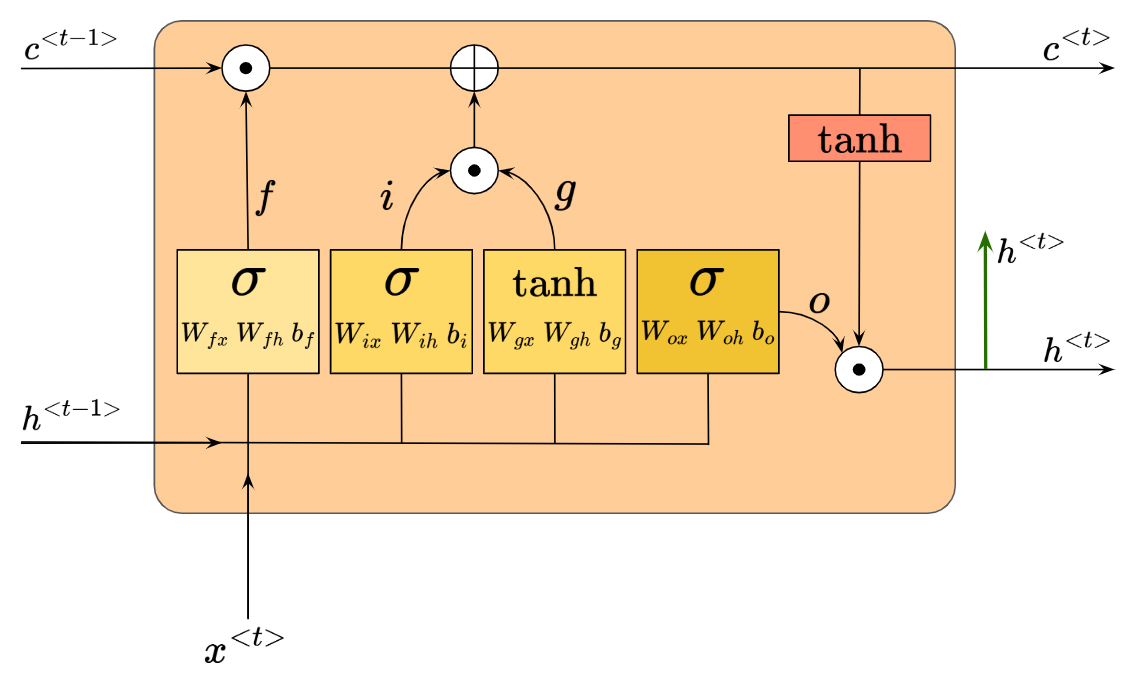
Notice the Weight and Bias inputs for each activation block within the cell. We also see the activated outputs, $f$, $i$, $g$ and $o$. We also see our usual $h^{<t-1>}$, $x^{<t>}$ & $h^{<t>}$ inputs and outputs. Finally, there’s also a new pair of I/O, in the form of $c^{<t-1>}$ and $c^{<t>}$.

$~ \\$

We’ll understand how the LSTM works by going through each core component. Let’s begin with the new I/O, $c^{<t-1>}$ and $c^{<t>}$.

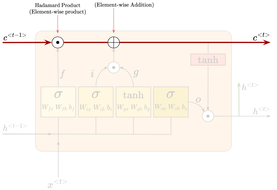
This component, called the ‘cell state’, is actually the key to the LSTM architecture. It is shown as a horizontal line passing through the top of the LSTM cell, and it only goes through two minor linear interactions (as seen from the white pieces).

The cell state passes information through, and the LSTM has the ability to add or remove information to the cell state, via the linear interactions mentioned above.

$~ \\$

LSTMs control the addition and removal of information through ‘gates’. They are composed out of a sigmoid neural net layer, and a hadamard product (or, element-wise multiplication operation).

Let’s walk through each of these gates, and along the way we’ll understand intuitively how they control information flow with the sigmoid activation.

$~ \\$

We’ll begin with the ‘Forget Gate’. It’s called the Forget Gate because it decides what information we will forget, or remove, from the cell state. It looks like this:

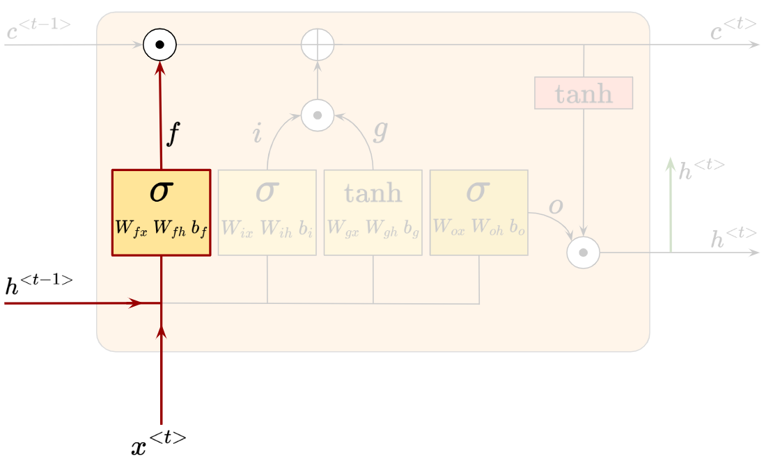
The sigmoid layer takes in $h^{<t-1>}$ and $x^{<t>}$, then outputs $f$, whereby:

$\boxed{f_t = \sigma( W_{fx} x^{<t>} + W_{fh} h^{<t-1>} + b_f)}$

The Forget Gate’s output $f_t$ has the same dimensionality as the previous cell state $C_{t-1}$. Since $f_t$ involves the sigmoid activation function, all of its values are forced between 0 and 1. Then, an element-wise multiplication happens between $c_{t-1}$ and $f_t$.

Let’s try to understand intuitively why this sigmoid activation and element-wise multiplication helps us decide what information to get rid of and what to keep.

Given a matrix representing the values in cell state $C_{t-1}$, and a matrix representing the values in $f_t$, here’s how the element-wise multiplication might look like:

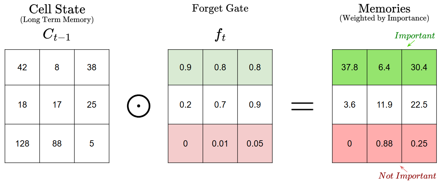
We can see that the matrix values in $f_t$ function as “weight” values, with larger values representing higher importance, and smaller values representing lower importance. “1” would mean to completely keep the corresponding information, and “0” would mean to completely get rid of the information. So, the element-wise multiplication weights the “memory” values in the cell state, which then helps us decide what memories to keep and discard.

Since the sigmoid values are between 0 and 1, the multiplication operation really mostly helps us lower the importance of select pieces of information, hence why this section is called the Forget Gate.

Now that we know how the Forget Gate works, let’s move on to the next section, involving the Input Gate and Input Node.

$~ \\$

Here’s how the Input Gate (red) and Input Node (green) look like:

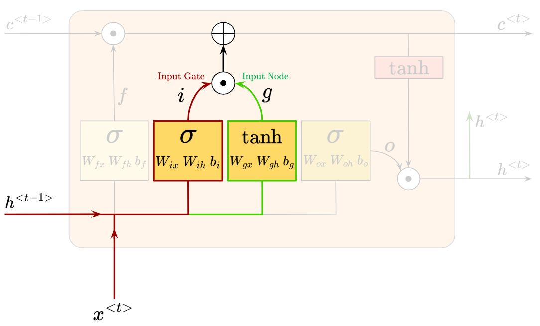
Whereby we have:

$\boxed{i_t = \sigma( W_{ix} x^{<t>} + W_{ih} h^{<t-1>} + b_i)} \\ ~ \\ \boxed{g_t = \tanh( W_{gx} x^{<t>} + W_{gh} h^{<t-1>} + b_g)} \\ ~ \\$

As we’ve seen from the sigmoid activation, the values of $i_t$ will be squeezed between 0 and 1. Meanwhile, the values of $g_t$ will be between -1 and 1, thanks to the tanh activation.

$i_t$ and $g_t$ go through the element-wise multiplication, then the result is added element-wise to our cell state.

Let’s try and imagine how $i_h$ and $g_t$ work, in a similar manner to how we understood the Forget Gate.

The Input Node $g_t$ is computed as $g_t$ = $tanh(W_{gx} x^{<t>} + W_{gh} h^{<t-1>} + b_g)$ and produces values between -1 and 1. The positive values reinforce a certain memory, while the negative values represent an opposing adjustment to the selected memory value. So, we can think of the input node as raw suggestions for what should be remembered or adjusted in the cell state.
The Input Gate $i_t$, which has a sigmoid activation, produces values between 0 and 1. Similarly to the Forget Gate, these values act as “importance weights”.
Now, we do the element-wise multiplication of $i_t$ and $g_t$, which produces a matrix containing positive and negative values, weighted by their importance.
Finally, we do an element-wise addition of ($i_t ⊙ g_t$) to our cell state.

Therefore, the Input Node and Input Gate work together to introduce new information to our cell state, and also modify existing information. The positive values represent new information, while negative values represent corrective updates to the existing memory. If we did not have negative values from $\text{tanh}$, LSTMs would only ever “increase” memory, never correct or reduce it.

$~ \\$

After going through the Forget Gate, Input Gate and Input Node, we actually have our new cell state, $C^{<t>}$. To summarize all the operations so far:

$\boxed{C^{<t>} = (C^{<t-1>} ⊙ f_t) ⊕ (i_t ⊙ g_t)}$

We can see how $f_t$, $i_t$ and $g_t$ have contributed to the new cell state $C^{<t>}$.

$~ \\$

Finally, we need to understand how the Output Gate updates the value of the hidden units, to produce $h^{<t>}$.

The relevant parts are highlighted, with the output gate in red:

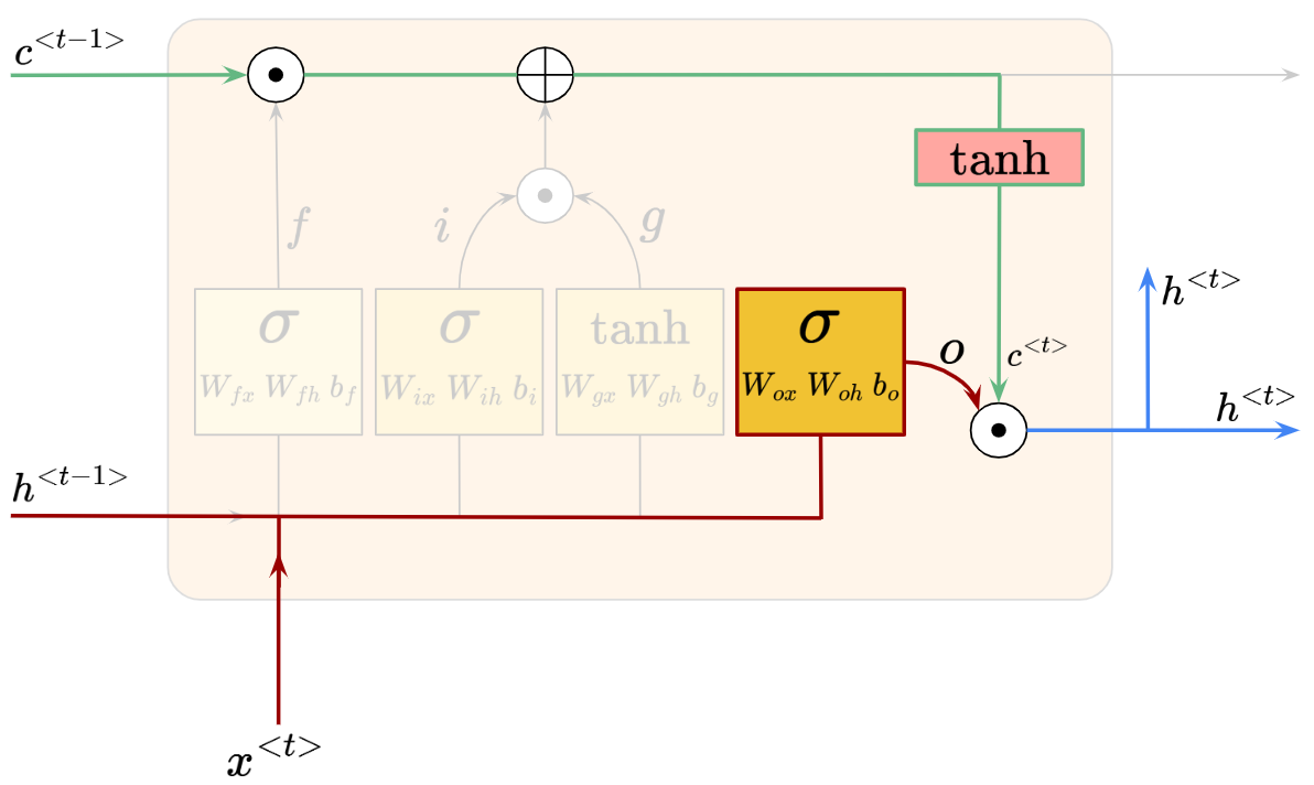
The output gate produces $O_t$, which is simply:

$\boxed{O_t = \sigma( W_{ox} x^{<t>} + W_{oh} h^{<t-1>} + b_o)}$

Then, to obtain the intended updated hidden state $h^{<t>}$, we do the element-wise multiplication of $O_t$ and the tanh-activated updated cell state $C^{<t>}$, which is:

$\boxed{h^{<t>} = o_t ⊙ \tanh(C^{<t>})}$

The output gate $O_t$ in an LSTM controls how much of the cell state’s information should influence the next time step’s hidden state $h^{<t>}$. However, the raw cell state $C^{<t>}$ is activated with tanh first, before doing an element-wise multiplication with $O_t$.

The reason for the tanh activation of $C^{<t>}$ is because the cell state represents the long term memory of the LSTM, which can contain large values and accumulate information over time. Therefore, if $C^{<t>}$ was used directly as $h^{<t>}$, the hidden state might explode in magnitude and become unstable. That’s why the tanh activation function is used to regulate the range of values.

On the other hand, the reason why we need $O_t$ is to act as a matrix of “importance weights” again, to decide how much of $C^{<t>}$ we want to influence $h^{<t>}$. This allows us to optimize for only allowing relevant information to be passed on.

Now that we have $h^{<t>}$, we pass it onto the next layer (eg. the output layer $y^{<t>}$) and also the hidden layer in the next time step.

2. Forward Propagation

Let’s summarize everything we’ve learnt so far to describe the forward propagation through our LSTM cell:

$\text{Forget Gate}$:

$\boxed{f_t = \sigma( W_{fx} x^{<t>} + W_{fh} h^{<t-1>} + b_f)}$

$\text{Input Gate}$:

$\boxed{i_t = \sigma( W_{ix} x^{<t>} + W_{ih} h^{<t-1>} + b_i)}$

$\text{Input Node}$:

$\boxed{g_t = \tanh( W_{gx} x^{<t>} + W_{gh} h^{<t-1>} + b_g)}$

$\text{Cell State Update}$:

$\boxed{C^{<t>} = (C^{<t-1>} ⊙ f_t) ⊕ (i_t ⊙ g_t)}$

$\text{Output Gate}$:

$\boxed{O_t = \sigma( W_{ox} x^{<t>} + W_{oh} h^{<t-1>} + b_o)}$

$\text{Hidden State}$:

$\boxed{h^{<t>} = o_t ⊙ \tanh(C^{<t>})}$

Additionally, we need to remember that this is only for the LSTM cell. It exists as part of a larger recurrent neural network, like in this (simplified) illustration:

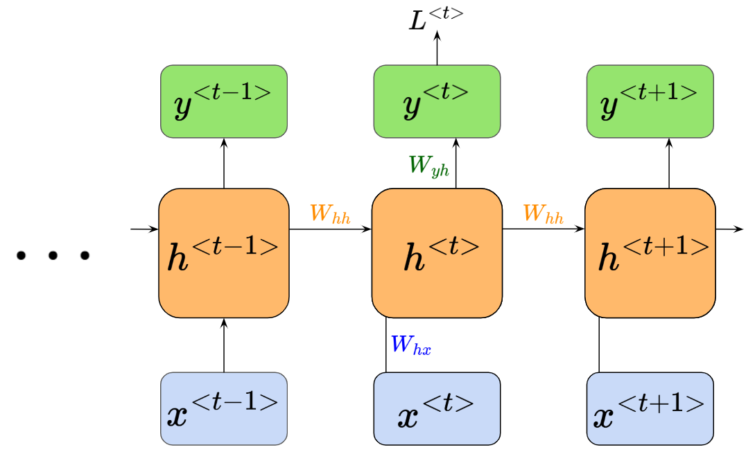
So, we need to account for:

$\boxed{z_y^{<t>} = W_{yh} h^{<t>} + b_y} \\ ~ \\ \boxed{\hat{y}^{<t>} = \sigma_y (z_y^{<t>})} \\ ~ \\$

2.1 Backward Propagation

This section will be a lot of math, with a lot overlapping from our previous derivation in the RNN post. Please feel free to skip past it!

Backpropagation from Output Layer to LSTM hidden state

Let our loss function be cross-entropy loss, where $L^{<t>} = - y^{<t>} \log (\hat{y}^{<t>})$.

Then, gradient of loss $L^{<t>}$ with respect to predicted value $\hat{y}^{<t>}$ is:

$\boxed{\frac{∂ L^{<t>}}{∂ \hat{y}^{<t>}} = -\frac{y^{<t>}}{\hat{y}^{<t>}}}$

Then, gradient of loss $L^{<t>}$ with respect to $z_y^{<t>}$:

$\boxed{\frac{∂ L^{<t>}}{∂ z_y^{<t>}} = \frac{∂ L^{<t>}}{∂ \hat{y}^{<t>}} \cdot \frac{∂ \hat{y}^{<t>}}{∂ z_y^{<t>}} = -\frac{y^{<t>}}{\hat{y}^{<t>}} \cdot \frac{∂ \text{ softmax}}{∂ z_y^{<t>}} = \hat{y}^{<t>} - y^{<t>}}$

Let’s find derivative of loss function with respect to weight $W_{yh}$:

$\boxed{\frac{∂ L^{<t>}}{∂ W_{yh}} = \frac{∂ L^{<t>}}{∂ z_y^{<t>}} \cdot \frac{∂ z_y^{<t>}}{∂ W_{yh}} = \frac{∂ L^{<t>}}{∂ z_y^{<t>}} \cdot \frac{∂ (W_{yh} h^{<t>} + b_y)}{∂ W_{yh}} = (\hat{y}^{<t>} - y^{<t>}) \cdot h^{<t>}}$

Also, the derivative of loss function with respect to bias $b_y$:

$\boxed{\frac{∂ L^{<t>}}{∂ b_y} = \frac{∂ L^{<t>}}{∂ z_y^{<t>}} \cdot \frac{∂ z_y^{<t>}}{∂ b_y} = \frac{∂ L^{<t>}}{∂ z_y^{<t>}} \cdot \frac{∂ (W_{yh} h^{<t>} + b_y)}{∂ b_y} = (\hat{y}^{<t>} - y^{<t>})}$

Next, crucially, we want to find derivative of loss function with respect to $h^{/}$:

$\boxed{\frac{∂ L^{<t>}}{∂ h^{<t>}} = \frac{∂ L^{<t>}}{∂ z_y^{<t>}} \cdot \frac{∂ z_y^{<t>}}{∂ h^{<t>}} = \frac{∂ L^{<t>}}{∂ z_y^{<t>}} \cdot \frac{∂ (W_{yh} h^{<t>} + b_y)}{∂ h^{<t>}} = (\hat{y}^{<t>} - y^{<t>}) \cdot W_{yh}}$

$~ \\$

Backpropagation through LSTM cell

$\text{Output Gate}$:

Given $h^{<t>} = o_t ⊙ \tanh(C^{<t>})$, we can find derivative of loss function with respect to $o_t$:

$\boxed{\frac{∂ L^{<t>}}{∂ o_t} = \frac{∂ L^{<t>}}{∂ h^{<t>}} \cdot \frac{∂ h^{<t>}}{∂ o_t} = \frac{∂ L^{<t>}}{∂ h^{<t>}} ⊙ \tanh(C^{<t>})}$

If we use $o_t = \sigma(z_o)$,

$\boxed{\frac{∂ L^{<t>}}{∂ z_o} = \frac{∂ L^{<t>}}{∂ o_t} ⊙ o_t ⊙ (1-o_t)}$

and we also have:

$\boxed{\frac{∂ L^{<t>}}{∂ W_{ox}} = \frac{∂ L^{<t>}}{∂ z_o} x^{<t>}} \\ ~ \\ \boxed{\frac{∂ L^{<t>}}{∂ W_{oh}} = \frac{∂ L^{<t>}}{∂ z_o} h^{<t-1>}} \\ ~ \\ \boxed{\frac{∂ L^{<t>}}{∂ b_o} = \displaystyle\sum \frac{∂ L^{<t>}}{∂ z_o}} \\ ~ \\$

Next, to find derivative of loss function with respect to $C^{<t>}$:

$\boxed{\frac{∂ L^{<t>}}{∂ C^{<t>}} = \frac{∂ L^{<t>}}{∂ h^{<t>}} \cdot ⊙ (1-\tanh(C^{<t>})) + \frac{∂ L^{<t+1>}}{∂ C^{<t+1>}} ⊙ f_{t+1}}$

Given $C^{<t>} = (C^{<t-1>} ⊙ f_t) ⊕ (i_t ⊙ g_t)$, we can find derivative of loss function with respect to each component!

$\text{Forget Gate}$:

$\boxed{\frac{∂ L^{<t>}}{∂ f_t} = \frac{∂ L^{<t>}}{∂ C^{<t>}} ⊙ C^{<t-1>}}$

If we use $f_t = \sigma(z_f)$,

$\boxed{\frac{∂ L^{<t>}}{∂ z_f} = \frac{∂ L^{<t>}}{∂ f_t} ⊙ f_t ⊙ (1-f_t)}$

and we also have:

$\boxed{\frac{∂ L^{<t>}}{∂ W_{fx}} = \frac{∂ L^{<t>}}{∂ z_f} x^{<t>}} \\ ~ \\ \boxed{\frac{∂ L^{<t>}}{∂ W_{fh}} = \frac{∂ L^{<t>}}{∂ z_f} h^{<t-1>}} \\ ~ \\ \boxed{\frac{∂ L^{<t>}}{∂ b_f} = \displaystyle\sum \frac{∂ L^{<t>}}{∂ z_f}} \\ ~ \\$

$\text{Input Gate}$:

$\boxed{\frac{∂ L^{<t>}}{∂ i_t} = \frac{∂ L^{<t>}}{∂ C^{<t>}} ⊙ g_t}$

If we use $i_t = \sigma(z_i)$,

$\boxed{\frac{∂ L^{<t>}}{∂ z_i} = \frac{∂ L^{<t>}}{∂ i_t} ⊙ f_t ⊙ (1-f_t)}$

and we also have:

$\boxed{\frac{∂ L^{<t>}}{∂ W_{ix}} = \frac{∂ L^{<t>}}{∂ z_i} x^{<t>}} \\ ~ \\ \boxed{\frac{∂ L^{<t>}}{∂ W_{ih}} = \frac{∂ L^{<t>}}{∂ z_i} h^{<t-1>}} \\ ~ \\ \boxed{\frac{∂ L^{<t>}}{∂ b_i} = \displaystyle\sum \frac{∂ L^{<t>}}{∂ z_i}} \\ ~ \\$

$\text{Input Node}$:

$\boxed{\frac{∂ L^{<t>}}{∂ g_t} = \frac{∂ L^{<t>}}{∂ C^{<t>}} ⊙ i_t}$

If we use $g_t = \tanh(z_g)$,

$\boxed{\frac{∂ L^{<t>}}{∂ z_g} = \frac{∂ L^{<t>}}{∂ g_t} ⊙ (1-C^{<t>})^2}$

and we also have:

$\boxed{\frac{∂ L^{<t>}}{∂ W_{gx}} = \frac{∂ L^{<t>}}{∂ z_g} x^{<t>}} \\ ~ \\ \boxed{\frac{∂ L^{<t>}}{∂ W_{gh}} = \frac{∂ L^{<t>}}{∂ z_g} h^{<t-1>}} \\ ~ \\ \boxed{\frac{∂ L^{<t>}}{∂ b_g} = \displaystyle\sum \frac{∂ L^{<t>}}{∂ z_g}} \\ ~ \\$

Finally, we’ll finish off the backpropagation section by summarizing how we update all the parameters based on the gradients of the current time step $t$:

Updating Output(y) Layer Parameters

$W_{yh} = W_{yh} - \alpha \cdot \frac{∂ L^{<t>}}{∂ W_{yh}} \\ b_y = b_y - \alpha \cdot \frac{∂ L^{<t>}}{∂ b_y} \\ ~ \\$

Updating Forget Gate Parameters

$W_{fx} = W_{fx} - \alpha \cdot \frac{∂ L^{<t>}}{∂ W_{fx}} \\ W_{fh} = W_{fh} - \alpha \cdot \frac{∂ L^{<t>}}{∂ W_{fh}} \\ b_f = b_f - \alpha \cdot \frac{∂ L^{<t>}}{∂ b_f} \\ ~ \\$

Updating Input Gate Parameters

$W_{ix} = W_{ix} - \alpha \cdot \frac{∂ L^{<t>}}{∂ W_{ix}} \\ W_{ih} = W_{ih} - \alpha \cdot \frac{∂ L^{<t>}}{∂ W_{ih}} \\ b_i = b_i - \alpha \cdot \frac{∂ L^{<t>}}{∂ b_i} \\ ~ \\$

Updating Input Node Parameters

$W_{gx} = W_{gx} - \alpha \cdot \frac{∂ L^{<t>}}{∂ W_{gx}} \\ W_{gh} = W_{gh} - \alpha \cdot \frac{∂ L^{<t>}}{∂ W_{gh}} \\ b_g = b_g - \alpha \cdot \frac{∂ L^{<t>}}{∂ b_g} \\ ~ \\$

Updating Output Gate Parameters

$W_{ox} = W_{ox} - \alpha \cdot \frac{∂ L^{<t>}}{∂ W_{ox}} \\ W_{oh} = W_{oh} - \alpha \cdot \frac{∂ L^{<t>}}{∂ W_{oh}} \\ b_o = b_o - \alpha \cdot \frac{∂ L^{<t>}}{∂ b_o} \\ ~ \\$

Phew. That was a lot! The working was done in my head, reading off latex code, so there may be some small mistakes or typos in there :P

2.2 How LSTMs Solve Vanishing/Exploding Gradients

It is commonly said that LSTMs are an improvement over RNNs in big part due to their ability to avoid the Vanishing/Exploding gradient problem.

We put a lot of effort to understand the effect of the sigmoid and tanh activation functions within the LSTM cell, and it will come in handy for understanding how LSTMs avoid the gradient problem.

The cell state $C_t$ allows information to flow largely unchanged across many time steps
This is because the cell state updates via element-wise additions rather than repeated multiplications (as in standard RNNs), gradients do not change exponentially.
The sigmoid and tanh functions in gating keep values bounded

Additionally, if gradients do grow too large, LSTMs often use gradient clipping!

3. Code Implementation

Finally, to the fun part. Due to the tedious steps shown above for the forward and backwards passes, we’ll implement the LSTM model with Pytorch instead.

import torch
import torch.nn as nn
import torch.optim as optim
import numpy as np

# Data I/O
data = open('bieber_dataset_cleaned.txt', 'r').read()
chars = list(set(data))
char_to_ix = {ch: i for i, ch in enumerate(chars)}
ix_to_char = {i: ch for i, ch in enumerate(chars)}

vocab_size = len(chars)
hidden_size = 512  # Hidden state size
num_layers = 3  # Two-layer LSTM
seq_length = 25  # Sequence length
learning_rate = 2e-3  # Learning rate
batch_size = 64  # Batch size

device = torch.device("cuda" if torch.cuda.is_available() else "cpu")

# Define LSTM model
class CharLSTM(nn.Module):
    def __init__(self, vocab_size, hidden_size, num_layers):
        super(CharLSTM, self).__init__()
        self.hidden_size = hidden_size
        self.num_layers = num_layers
        
        self.embed = nn.Embedding(vocab_size, hidden_size)
        self.lstm = nn.LSTM(hidden_size, hidden_size, num_layers, batch_first=True)
        self.fc = nn.Linear(hidden_size, vocab_size)
    
    def forward(self, x, hidden):
        x = self.embed(x)  # Convert to embeddings
        out, hidden = self.lstm(x, hidden)
        out = self.fc(out.reshape(out.size(0) * out.size(1), out.size(2)))
        return out, hidden
    
    def init_hidden(self, batch_size):
        return (torch.zeros(self.num_layers, batch_size, self.hidden_size).to(device),
                torch.zeros(self.num_layers, batch_size, self.hidden_size).to(device))

# Initialize model, loss, and optimizer
model = CharLSTM(vocab_size, hidden_size, num_layers).to(device)
criterion = nn.CrossEntropyLoss()
optimizer = optim.Adam(model.parameters(), lr=learning_rate)

# Training loop
num_epochs = 5000  # Number of iterations
hprev = model.init_hidden(batch_size)

for epoch in range(num_epochs):
    if (epoch * seq_length + seq_length >= len(data)):
        hprev = model.init_hidden(batch_size)  # Reset hidden state
        start = 0
    else:
        start = epoch * seq_length
    
    inputs = []
    targets = []

    for i in range(batch_size):
        start_idx = (epoch * seq_length + i * seq_length) % (len(data) - seq_length)
        input_seq = [char_to_ix[ch] for ch in data[start_idx:start_idx+seq_length]]
        target_seq = [char_to_ix[ch] for ch in data[start_idx+1:start_idx+seq_length+1]]
        
        inputs.append(input_seq)
        targets.append(target_seq)

    inputs = torch.tensor(inputs, dtype=torch.long).to(device)  # Shape: (batch_size, seq_length)
    targets = torch.tensor(targets, dtype=torch.long).to(device)  # Shape: (batch_size, seq_length)

    
    model.zero_grad()
    hprev = tuple([h.detach() for h in hprev])
    outputs, hprev = model(inputs, hprev)
    loss = criterion(outputs, targets.view(-1))
    loss.backward()
    optimizer.step()
    
    if epoch % 100 == 0:
        print(f'Epoch [{epoch}/{num_epochs}], Loss: {loss.item():.4f}')
        
        # Sample text
        sample_input = torch.tensor([char_to_ix[data[start]]], dtype=torch.long).unsqueeze(0).to(device)
        h_sample = model.init_hidden(1)
        sampled_chars = []
        
        for _ in range(200):  # Generate 200 characters
            output, h_sample = model(sample_input, h_sample)
            prob = torch.nn.functional.softmax(output[-1], dim=0).detach().cpu().numpy()
            char_index = np.random.choice(vocab_size, p=prob)
            sampled_chars.append(ix_to_char[char_index])
            sample_input = torch.tensor([[char_index]], dtype=torch.long).to(device)
        
        print("----\n" + ''.join(sampled_chars) + "\n----")

$~ \\$

Here are the results at various iterations:

Iteration 100, Loss: 1.6708

ls yor hares.
Wut firnsty, sir. his fnor,
Whasry tneash,
Hhi, rity that hy esilk arh to btirely

MNNREINS:
Sey cood afcirssest to if im prowets ally

MitiEhithe the dide ade 'rone unot onith the the y

Iteration 1000, Loss: 0.3475

&n; graiply hers worn woulds that and fure
aforitiue.

CORIOLANUS:
What these are to her humble weld,
Hew your them aon: had mafeed and him.

COMINIUS:
Not all in of amgin, whem suf'er.

Iteration 3000, Loss: 0.3289

aman'Nt, shail her bay.

KING RICHARD III:
You speak too bitterly.

DUCHESS OF YORK:
Hear me a word;
For I, that scomfort, thou know'st, that reach of long
To be slaze them safety of your grace makes 

It seems like the LSTM performs much better than the RNN we made previously, though we definitely made a much more comprehensive model (much larger hidden size, 3x more layers, longer sequence length and batching the updates).

In my experimentation, I found that having a longer sequence length reduced the amount of memorization and sentences being printed verbatim from the dataset. Batching also improved the loss optimization a lot!

That’s all for this project, thanks for reading!

References

The writing in this post borrows heavily from the excellent writing by Christopher Olah.

I also referenced and modified many illustrations from this slide deck by Sebastian Raschka. He also happens to be a favourite author :D

The dataset was also obtained from the repo linked in Andrej Karpathy’s blog post here.