Building a Neural Network from scratch
In this project, I build an image classifying neural network using only NumPy and some math.
In this project, we’re going to build a simple neural network from scratch, using NumPy.
We’ll build a shallow 2-layer neural network (one hidden and one output). This neural network will be trained on data from the MNIST handwritten digit dataset, and classify input images to digits.
The MNIST dataset consists of 28x28 grayscale images of handwritten digits. Each image is labelled with the digit it belongs to.
Here’s the structure for this project post:
1. Neural Network Overview
2. Describing the Neural Network Mathematically
2.1 Forward Propagation
2.2 Backward Propagation
2.2.1 Deriving $dA^{[2]}$
2.2.2 Deriving $dZ^{[2]}$
2.2.3 Deriving $dW^{[2]}$
2.2.4 Deriving $db^{[2]}$
2.2.5 Deriving $dZ^{[1]}$
2.2.6 Deriving $dW^{[1]}$ and $db^{[1]}$
2.3 Section 2 Summary
3. Code Implementation
1. Neural Network Overview
Our Neural Network will have three layers in total - an input layer, a hidden layer and an output layer.
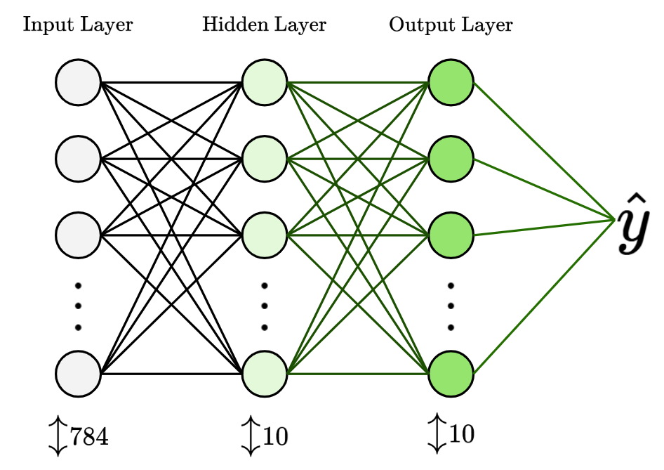
The input layer has 784 nodes, which corresponds to the total number of pixels in each 28x28 input image from the MNIST dataset. Each pixel is described by a value between [0,255], which represents pixel intensity (white being 255, black being 0).
Next, to keep things simple, we’ll give the hidden layer 10 nodes. The value of these nodes is first calculated based on the weights and biases applied to the 784 nodes from the input layer, followed by a ReLU activation function.
Finally, the output layer will have 10 nodes, which corresponds to each output class. We have 10 possible digit values (0 to 9), so we have 10 output classes. The value of these nodes are first calculated based on the weights and biases applied to the 10 nodes from the hidden layer, followed by a Softmax activation function.
Then, the output layer will give us a column of 10 probability values, containing a value between [0,1] for each class.
We’ll then classify the image based on the digit class with the highest probability value.
2. Describing the Neural Network Mathematically
In this section, we will formalize our neural network mathematically, so that we can reproduce relevant variables in code later.
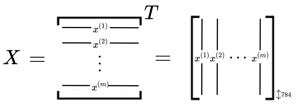
We'll begin by understanding the dimensionality of our input data.
Conventionally, our input data would stack the information for each image as rows of a matrix. However, because we will be doing matrix multiplication with weights, we’ll transpose the conventional matrix to obtain our matrix $X$, which has image data as columns instead. Thus, matrix $X$ would have columns of height $784$, with $m$ total columns (where our input dataset has $m$ images, for example).
Next, we'll look at the weights and biases between our neural network layers.
Let’s index our layers like so: the input layer is layer 0, hidden layer is layer 1 and output layer is layer 2.
Between each pair of layers is a set of connections between every node in the previous node and every node in the following one. When values from one layer get passed to the next layer, there is a weight applied to each node value from the original layer, followed by a bias term added to the weighted node value. Finally, there will be an activation function applied to the weighted and biased node value, to add non-linearity to the output.
Mathematically, we would describe it like this:
Let’s say we’re going from layer 0 (784 nodes) to layer 1 (10 nodes). Each node $h_i$ in layer 1 is computed as:
Where:
- $x_j$ is the input value from originating node $j$
- $w_ij$ is the weight connecting input node $j$ to node $i$
- $b_i$ is the bias applied to node $i$
- $f(\cdot)$ is the activation function (eg. ReLU, sigmoid, tanh)
Let’s call the weight matrix connecting layer 0 to layer 1 as $W^{[1]}$. Our weight matrices are of dimension $n^L \times n^{(L-1)}$, where $n^{(L-1)}$ is the number of nodes in the originating layer, while $n^L$ is the number of nodes in the receiving layer.
For example, $W^{[1]}$ would be a $10 \times 784$ matrix, while $W^{[2]}$ would be a $10 \times 10$ matrix.
Next, for biases, we know that they’re simply constant terms added to each weighted node in the receiving layer. So, biases are represented as a $n^L$-dimensional vector. Let’s call the bias vector connecting layer 0 to layer 1 as $b^{[1]}$.
For example, both $b^{[1]}$ and $b^{[2]}$ would be 10-dimensional vectors.
Moving on to the next section, we’ll formulate the mathematical operations that happen during the forward propagation phase of our neural network.
2.1 Forward Propagation
During the forward propagation, we know that weights, biases and activation functions are applied to our data.
Let's cover the mathematical operations going from layer 0 to layer 1:
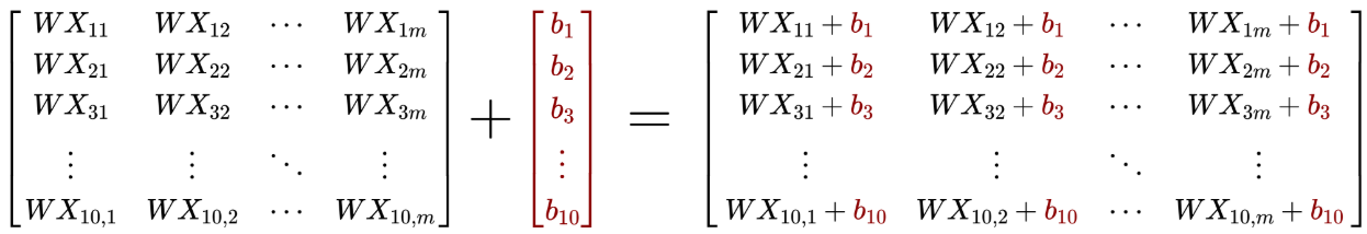
For our input data matrix $X$, we’ll apply weight matrix $W^{[1]}$ and bias matrix $b^{[1]}$, such that we obtain the un-activated output $Z^{[1]}$:
$W^{[1]}$ has dimensions $10 \times 784$, while $X$ has dimensions $784 \times m$, so $W^{[1]}X$ has dimensions $10 \times m$. We then add the $10$-dimensional vector $b^{[1]}$ to every column in $W^{[1]}X$, like so:
Next, we’ll apply the Rectified Linear Unit (ReLU) activation function to $Z^{[1]}$. ReLU is a simple function that adds non-linearity to our neural network, like so:
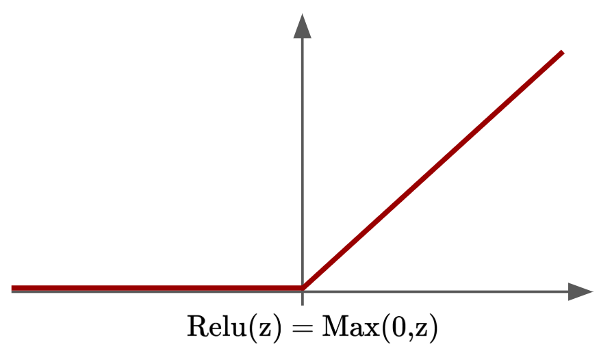
So, when adding ReLU to $Z^{[1]}$, we’ll call the ReLU function $g^{[1]}$ and the output $A^{[1]}$, whereby:
Next, we'll cover the mathematical operations going from layer 1 to layer 2:
We’ll now apply the weights and biases going from layer 1 to 2, whereby:
Then, we’ll apply the Softmax activation function to $Z^{[2]}$ to get the final output. If we had more hidden layers, we could use something like ReLU, but since it is the output layer, we specially need the Softmax activation function.
This is because for each column in $Z$, Softmax exponentiates each individual column entry, then divides each exponentiated entry by the sum of all exponentiated entries in the column.
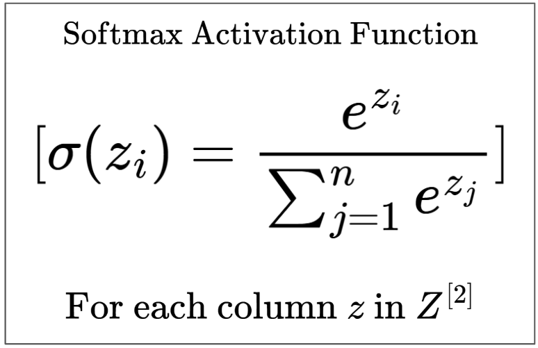
This ensures we have a output values in the range (0,1) that sum to 1, thus making them interpretable as probabilities. This is necessary for our image classification task.
So, for Softmax function $g^{[2]}$, we have:
Now that we’ve covered the final layer, we’ve run through the entire forward propagation through the neural network. Next, we’ll cover backward propagation.
2.2 Backward Propagation
We need to do backpropagation in order to carry out gradient descent and make our neural network “learn”.
Mathematically, what we’re computing is the derivative of the loss function with respect to each weight and bias parameter, which allows us to identify the contribution of each parameter to our total loss, which enables us to update/optimize them accordingly.
Let's begin by choosing a suitable loss function:
Since we’re using the Softmax activation function, we’ll use Cross-Entropy Loss (also called log loss), whereby for a given column:
Where class label $y$ is the one-hot encoded ground truth (only one class is 1, rest are 0), and $\hat{y}$ is the predicted probability.
Since the ground truth $y$ is one-hot encoded, the loss value simplifies to:
Where $c$ is the correct class index. The closer $y_c$ is to 1, the closer the loss is to 0. The closer $y_c$ is to 0, the more loss approaches $+\infty$.
So, by minimizing the loss function, we improve the accuracy of our model.
Next, let's go over the gradient descent and backpropagation phase detail:
To minimize the loss, we update each parameter by subtracting the learning rate $\alpha$ times the derivative of the loss function with respect to that parameter. We repeat this process over many rounds of gradient descent. This allows us to converge toward a set of parameters that minimize the total loss.
So, gradient descent process would look something like this:
Therefore, our objective is to find the derivatives $\frac{∂J}{∂ W^{[1]}}$, $\frac{∂J}{∂ b^{[1]}}$, $\frac{∂J}{∂ W^{[2]}}$ and $\frac{∂J}{∂ b^{[2]}}$.
Let’s make things simpler and label these values as $dW^{[1]}$, $db^{[1]}$, $dW^{[2]}$ and $db^{[2]}$ respectively.
To find each of these values, we need to step backwards through our network, starting with $\frac{∂J}{∂ A^{[2]}}$, also labelled as $dA^{[2]}$, since that was the final output.
2.2.1 Deriving $dA^{[2]}$
Let's do some quick math to derive $dA^{[2]}$:
By considering a single data point in $\hat{y}$ first:
Then, if we generalize to all data points in the vectors $y$ and $\hat{y}$:
Finally, we obtain:
2.2.2 Deriving $dZ^{[2]}$
We find $dZ^{[2]}$ like so:
Okay, seems like to find $dZ^{[2]}$, we need to first find the derivative of the Softmax output $A^{[2]}$ with respect to $Z^{[2]}$. Crud. Let’s just get into it, but we’ll substitute $Z^{[2]}$ with “$x$” for now, to avoid latex notation hell for me :P
Let’s proceed to compute $\frac{∂ A^{[2]}_i}{∂ x_j}$ for some arbitrary $i$ and $j$:
Observe that:
Similarly:
Therefore, in the case that $i = j$ (like in the diagonal of the jacobian matrix):
Similarly, in the case that $i \ne j$:
To summarize:
And to go back to our original task of finding $dZ^{[2]}$:
Finally, for all elements of $Z^{[2]}$, we have:
2.2.3 Deriving $dW^{[2]}$
Now, we want to find $dW^{[2]}$. Using the chain rule again, we can do:
Since we know that $Z^{[2]} = W^{[2]} A^{[1]} + b^{[2]}$, we have:
Hence, we have:
2.2.4 Deriving $db^{[2]}$
Now, we want to find $db^{[2]}$. Using the chain rule again, we can do:
Since we know that $Z^{[2]} = W^{[2]} A^{[1]} + b^{[2]}$, we have:
Hence, we have:
2.2.5 Deriving $dZ^{[1]}$
Now, we want to find $dZ^{[1]}$. Using the chain rule, we can do:
Since we know that $Z^{[2]} = W^{[2]} A^{[1]} + b^{[2]}$, we can find $\frac{∂ Z^{[2]}}{∂ A^{[1]}}$:
Next, we need to find $\frac{∂ A^{[1]}}{∂ Z^{[1]}}$. Since $A^{[1]} = g_{ReLU}(Z^{[1]})$:
Thankfully the gradient for ReLU was easy to derive.
Putting it all together, we have:
Note that we need to use the Hadamart product operation $\odot$ because ReLU was applied element-wise on $Z^{[1]}$, and the same must apply going backwards.
2.2.6 Deriving $dW^{[1]}$ and $db^{[1]}$
Recall that $Z^{[1]} = W^{[1]} X + b^{[1]}$. We will use similar techniques in earlier sections to find our last two variables, $dW^{[1]}$ and $db^{[1]}$.
We begin with:
We also have:
Note that $dW^{[1]}$ finds gradient of the loss function with respect to the weight matrix, but $d^{[1]}$ is simply the average of the error terms $dZ^{[1]}$ because the bias term is shared across all examples in the batch, and it affects all neurons in the first layer equally.
2.3 Section 2 Summary
Let’s now summarise all the variables we’ve derived for the forward and backward propagation, along with the parameter update mechanism:
$\text{Forward Propagation:}$
$\text{Backward Propagation:}$
$\text{Parameter Updates:}$
Where $\alpha$ is the learning rate that we need to define/tune.
So, to recap, when running the neural network model:
1. First, we carry out forward propagation, and get a prediction for a given input image:
2. Then, we carry out backpropagation to compute loss function derivatives:
3. Finally, we update our parameters accordingly:
4. Then, we repeat this process over and over again (possibly up to an exact number of times, based on an iteration count limit that we set ourselves), until we are satisfied with the performance of our model (this could also be a limit defined by us).
3. Code Implementation
We’ll begin the code implementation by importing our packages and data.
We’re accessing the MNIST dataset from the ‘train.csv’ file provided by the ‘digit-recognizer’ kaggle page.
import numpy as np
import pandas as pd
from matplotlib import pyplot as plt

data = pd.read_csv('digit-recognizer/train.csv')
Next, we’ll do some basic data processing.
The data comes in as a 42000 x 785 matrix, where the first column contains the digit label, and the other 784 columns contain pixel intensity values. There are 42000 rows, representing 42000 training images.
We’ll also be scaling down the pixel intensity values in our x_train and x_test sets to fit in the range [0,1].
data = np.array(data)                # 42000 x 785
m,n = data.shape
np.random.shuffle(data)

data_test = data[0:1000].T           # 785 x 1000
y_test = data_test[0]                # 1 x 1000
x_test = data_test[1:n] / 255.0      # 784 x 1000

data_train = data[1000:m].T          # 785 x 41000
y_train = data_train[0]              # 1 x 41000
x_train = data_train[1:n] / 255.0    # 784 x 41000
Next, we’ll write a bunch of helper functions to do the computations required during forward propagation, backward propagation and parameter updating.
Additionally, we will scale down the weights to prevent crazy gradient values, and simply initialize biases to zero.
def init_params():
    W1 = np.random.rand(10,784) * 0.01
    b1 = np.zeros((10,1))
    W2 = np.random.rand(10,10) * 0.01
    b2 = np.zeros((10,1))
    return W1, b1, W2, b2

def ReLU(Z):
    return np.maximum(Z,0)

def softmax(Z):
    Z -= np.max(Z, axis=0)
    A = np.exp(Z) / np.sum(np.exp(Z), axis=0)
    return A

def forward_prop(W1, b1, W2, b2, X):
    Z1 = W1.dot(X) + b1
    A1 = ReLU(Z1)
    Z2 = W2.dot(A1) + b2
    A2 = softmax(Z2)
    return Z1, A1, Z2, A2

def ReLU_deriv(Z):
    return Z > 0

def one_hot(Y):
    one_hot_Y = np.zeros((Y.size, Y.max() + 1))
    one_hot_Y[np.arange(Y.size), Y] = 1
    one_hot_Y = one_hot_Y.T
    return one_hot_Y

def backward_prop(Z1, A1, Z2, A2, W1, W2, X, Y):
    m = X.shape[1]
    one_hot_Y = one_hot(Y)
    dZ2 = A2 - one_hot_Y
    dW2 = (1 / m) * dZ2.dot(A1.T)
    db2 = (1 / m) * np.sum(dZ2)
    dZ1 = W2.T.dot(dZ2) * ReLU_deriv(Z1)
    dW1 = (1 / m) * dZ1.dot(X.T)
    db1 = (1 / m) * np.sum(dZ1)
    return dW1, db1, dW2, db2

def update_params(W1, b1, W2, b2, dW1, db1, dW2, db2, alpha):
    W1 = W1 - alpha * dW1
    b1 = b1 - alpha * db1
    W2 = W2 - alpha * dW2
    b2 = b2 - alpha * db2
    return W1, b1, W2, b2
Next, we’ll write some simple functions to help with finding model accuracy, and run the entire gradient descent process.
def get_predictions(A2):
    return np.argmax(A2, axis=0)  # argmax with axis=0 returns index of max value entry for every column

def get_accuracy(predictions, Y):
    return (np.sum(predictions == Y) / Y.size) * 100

def gradient_descent(X, Y, alpha, iterations):
    W1, b1, W2, b2 = init_params()

    for i in range(iterations):
        Z1, A1, Z2, A2 = forward_prop(W1, b1, W2, b2, X)
        dW1, db1, dW2, db2 = backward_prop(Z1, A1, Z2, A2, W1, W2, X, Y)
        W1, b1, W2, b2 = update_params(W1, b1, W2, b2, dW1, db1, dW2, db2, alpha)

        if i % 50 == 0:
            print("Iteration: ", i)
            predictions = get_predictions(A2)
            print(f"Accuracy: {get_accuracy(predictions, Y):.2f}%")
            print("")

    return W1, b1, W2, b2
Now, let’s finally train our model!
W1, b1, W2, b2 = gradient_descent(x_train, y_train, 0.1, 501)
Iteration:  0
Accuracy: 11.19%

Iteration:  50
Accuracy: 9.82%

Iteration:  100
Accuracy: 17.00%

Iteration:  150
Accuracy: 39.05%

Iteration:  200
Accuracy: 59.57%

Iteration:  250
Accuracy: 79.29%

Iteration:  300
Accuracy: 83.61%

Iteration:  350
Accuracy: 85.71%

Iteration:  400
Accuracy: 86.97%

Iteration:  450
Accuracy: 87.89%

Iteration:  500
Accuracy: 88.46%
So, we get roughly 88% accuracy on our train set.
Next, let’s see how our model performs on the test set.
We’ll do forward propagation through the test set, and see how well our predicted values test.
def make_predictions(X, W1, b1, W2, b2):
    _, _, _, A2 = forward_prop(W1, b1, W2, b2, X)
    predictions = get_predictions(A2)
    return predictions

test_set_predictions = make_predictions(x_test, W1, b1, W2, b2)

print(f"Test Set Accuracy: {get_accuracy(test_set_predictions, y_test):.2f}%")
Test Set Accuracy: 88.10%
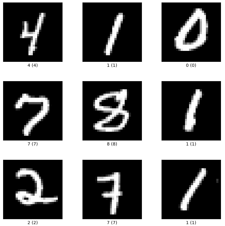
That’s pretty consistent! Glad to see our neural network is fitted decently well.
Finally, let’s visualize some sample images, their labels, and our predicted labels.
def visualize_test_prediction(index, W1, b1, W2, b2):
    current_image = x_test[:, index, None]
    prediction = make_predictions(current_image, W1, b1, W2, b2)
    label = y_test[index]
    print("Prediction: ", prediction)
    print("Label: ", label)

    current_image = current_image.reshape((28,28)) * 255
    plt.gray()
    plt.imshow(current_image, interpolation = 'nearest')
    plt.show()

visualize_test_prediction(0, W1, b1, W2, b2)
visualize_test_prediction(100, W1, b1, W2, b2)
visualize_test_prediction(17, W1, b1, W2, b2)
visualize_test_prediction(18, W1, b1, W2, b2)
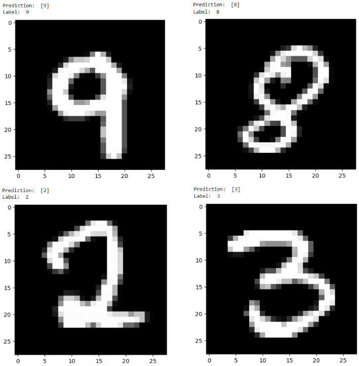
Nice! Project success.
Thanks for reading!
References
This project heavily references this kaggle notebook by Samson Zhang.
I also found Mustafa’s derivation of the Softmax function very helpful.