Building a Recurrent Neural Network (RNN) from scratch
In this project, I build a RNN using only NumPy and some math, and it will be used to generate text.
In this project, we’re going to build a simple recurrent neural network from scratch, using NumPy.
We’ll add a fun twist to this project by training the RNN on a dataset containing the written works by Shakespeare, and we’ll see how well it can generate new writing based on the learned patterns!
Given the foundational knowledge on neural networks established in previous projects, we’ll move relatively quickly into the theory for RNNs.
This project is also closely linked to the next one on Long Short-Term Memory (LSTM) networks, where we will improve on the RNN architecture.
Here’s the structure for this project post:
1. Recurrent Neural Network Overview
2. Describing the RNN mathematically
2.1 Forward Propagation
2.2 Backward Propagation
2.2.1 Deriving Components In Backpropagation Through Time
2.3 The Vanishing & Exploding Gradient Problem
3. Code Implementation & Results
1. Recurrent Neural Network Overview
Recurrent Neural Networks are a type of neural work designed for processing sequential data, such as text, audio, time-series data and more. As the name suggests, the key feature that makes RNNs unique is the presence of recursive computational loops that span adjacent time steps.
This recurrence enables RNN models to effectively maintain a persistent internal state or “memory” of prior inputs, which can inform the processing of data points later in the sequence.
You might recall that our basic neural network usually has at least an input layer, a hidden layer and an output layer. Here’s how the basic architecture of a RNN differs:

We can see that the RNN now introduces a recursive relationship somehow with $h^{<t>}$, and also introduces a dimension of time $t$ to its layers.
In the above diagram, the RNN structure consists of a single computational unit with the self-connected hidden state. However, we can actually ‘unfold’ this single computational unit to see how information cycles across timesteps:
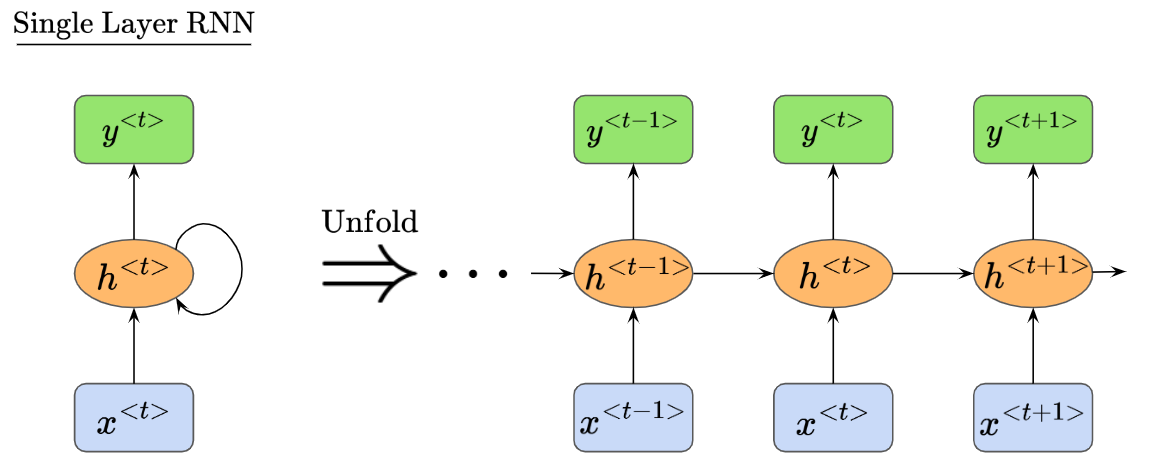
As data passes through the RNN, we can see how the input sequence is processed across all time steps, and how the model is influenced by information from previous time steps.

Hopefully it is also clear how each hidden unit $h^{<\cdots>}$ receives 2 inputs. For example, we see that $h^{<t>}$ receives two inputs colored in red, $h^{<t-1>}$ and $x^{<t>}$. Correspondingly, $h^{<t+1>}$ receives two inputs colored in purple, $h^{<t>}$ and $x^{<t+1>}$
You may also be wondering, how would a multi-layer RNN look like? It might be hard to imagine all the inputs and outputs moving about. It would look something like this:

There is also an important point to be made about parameter sharing in RNNs. Let’s say we have a classic feedforward neural network that is trained to predict the next character in English sentences (or text sequences). The feedforward net would require separate weights for each input-output mapping for every character position. Given two similar, but differently worded sentences:
- “Today, I went to the dentist”
- “I went to the dentist today”
The feedforward neural network would learn the contextual relationships completely independently, and thus relearn from scratch even if similar semantic patterns were seen before. It cannot develop a ‘unified grammar model’.
On the otherhand, the RNN shares the weights across certain time-steps, so if it learns patterns or rules in one part of a sentence, these can be reapplied later even if the sequence order changes slightly. More technically, the RNN embeds language patterns as reusable transition functions in the shared weights, so they are retained and applied regardless of input sequence length, or sentence order.
This means that for sequential data (like characters in a sentence), using RNNs can result in simpler models with fewer parameters to train while having better performance compared to a classic feedforward neural network.
Okay, now we’re ready to learn how a RNN works under the hood. We’ll proceed to describe the RNN operations mathematically.
2. Describing the RNN mathematically
In this section, we’ll understand the operations happening within the RNN mathematically.
Let’s begin by understanding what weight matrices get passed around in a single hidden layer RNN:

We can see that $h^{<t>}$ receives two weight matrices: $W_{hx}$ from $x$, and $W_{hh}$ from its past self.
Then, $h^{<t>}$ outputs a weight matrix $W_{yh}$ which is passed into $y^{<t>}$.
Let’s unfold this to see things more clearly:

Now, we have a bigger picture of how the weight matrices are passed around the RNN. However, as we know, neural networks usually have other components like bias terms, and activation functions that add non-linearity. We’ll understand the full picture of how these weight matrices are used to form the inputs to each node, in the next section.
2.1 Forward Propagation
Let’s start by focusing on the inputs to the hidden layer node $h^{<t>}$, labelled in dark red:

As mentioned, our RNN also has biases and activation functions. Here’s what the Net Input and Activation terms at node h look like:
$\text{Net Input to Node h:}$
$\text{Activation at Node h:}$
Usually, the activation function $\sigma_h$ used here is the $\text{tanh}$ function.
After passing the input $z_h^{<t>}$ through the activation function to obtain $h^{<t>}$, we will then use $h^{<t>}$ in subsequent operations as part of the input to $y^{<t>}$, and to the next hidden node $h^{<t+1>}$.
Next, let’s focus on the net input and outputs at our output node $y^{<t>}$, labelled in dark red:

$\text{Net Input to Node y:}$
$\text{Output at Node y:}$
Usually, the activation function $\sigma_y$ used here is the $\text{Softmax}$ function.
Surprisingly, this is pretty much it for our forward propagation!
We simply covered the inputs and outputs to node $h^{<t>}$, and the same for node $y^{<t>}$.
Next, let’s learn how backpropagation is done in RNNs.
2.2 Backward Propagation
Before we go into the details of backpropagation, we must first define the Loss function we’re optimizing for.
Let’s say we chose Cross-Entropy Loss as our loss function $L$.
Recall how we have an output at node $y^{<t>}$ which changes for each time step $t$? Therefore, the overall loss $L$ can be computed as the sum over all time steps, like so:

Then, the question is, given the variable nature of our time-dependent components, how do we do backpropagation? Well, in RNNs, we do something called Backpropagation Through Time (BTT).
It’s called BTT because we calculate the gradients in the backpropagation layer by layer, but specifically from the last time step towards the original time step. In other words, we’re going backwards in time, hence the name!
Let’s dive into the derivation of our BTT process next.
2.2.1 Deriving Components In Backpropagation Through Time
Starting with the loss function, which we defined as the cross-entropy loss:
Using the derivative of natural log, the derivative of the loss function with respect to predicted value $\hat{y}^{<t>}$ is:
Then, moving to the derivative of loss function with respect to weighted input $z_y^{<t>}$, using the derivative of the softmax formula (derived in my previous project post on basic neural networks):
Next, the weighted input $z_y^{<t>}$ is comprised of two components, the weight $W_{yh}$ and bias $b_y$.
Let’s find derivative of loss function with respect to weight $W_{yh}$:
Also, the derivative of loss function with respect to bias $b_y$:
The next layer down would be the activated function $h^{<t>} = \sigma_h (z_h^{<t>})$, where we want to find the derivative of loss function with respect to $h^{<t>}$.
However, recall that while activated function $h^{<t>}$ directly contributes to our output $\hat{y}^{<t>}$ at time step $t$, it is also passed into the activated function of the next time step, where $z^{<t+1>} = W_{hx} x^{<t+1>} + W_{hh} h^{<t>} + b_h$, which also propagates forward to all continuing time steps.
Hence, in order to find the total derivative of loss function with respect to $h^{<t>}$, we need to add the derivative of $L^{<t>}$ with respect to $h^{<t>}$ and the derivative of $L^{<t+1>}$ with respect to $h^{<t>}$.
We’ll start with derivative of $L^{<t>}$ with respect to $h^{<t>}$:
And also the derivative of $L^{<t+1>}$ with respect to $h^{<t>}$:
Adding both together, the total derivative of $L^{<t>}$ with respect to $h^{<t>}$ is:
Next, we’ll go deeper to find the derivative of our loss function with respect to weighted sum $z_h^{<t>}$. To do this, we’ll use the derivative of $\text{tanh}$:
Finally, since we know that $z_h^{<t>} = W_{hx} x^{<t>} + W_{hh} h^{<t-1>} + b_h$, we can finish BTT by finding the derivative of loss function with respect to $W_{hx}$, $W_{hh}$ and $b_h$.
Let’s start with derivative of loss function with respect to $W_{hx}$:
Next, to find the derivative of loss function with respect to $W_{hh}$:
Finally, we find the derivative of loss function with respect to $b_h$:
Nice! We’re finally done with the derivation for backpropagation through time.
Just a quick note, recall that $\frac{∂ L^{<t>}}{∂ h^{<t>}}$ is dependent on $\frac{∂ L^{<t+1>}}{∂ h^{<t>}}$, and in the same way, $\frac{∂ L^{<t-1>}}{∂ h^{<t-1>}}$ will be dependent on $\frac{∂ L^{<t>}}{∂ h^{<t-1>}}$.
The derivative of our loss function $L^{<t>}$ with respect to $h^{<t-1>}$ is:
We will store the value in a variable so that it can be updated every time step $t$ and used for calculation in the next time step $t-1$.
Finally, let’s summarize how we update all the parameters based on the gradients of current time step $t$:
2.3 The Vanishing & Exploding Gradient Problem
Did you notice that for our above derivation of the loss function with respect to $W_{hh}$:
The result involves $h^{<t-1>}$?
Let’s consider the hidden state update rule:
Since $h^{<t>}$ depends on $h^{<t-1>}$, and $h^{<t-1>}$ itself depends on $h^{<t-2>}$ and so on, we get a recursive dependency.
Since each hidden state depends on the previous hidden state, if we modify $h^{<k>}$, it will not just affect $h^{<k+1>}$ but all future states $h^{<k+2>}$ and so on. Thus, to compute how much $h^{<t>}$ changes with respect to $h^{<k>}$, we must recursively track how each hidden state depends on the previous one.
This also means that the effect of $W_{hh}$ at time step $t$ is not just through its direct contribution at time $t$, but indirectly through all previous hidden states $h^{<k>}$ where $k \lt t$.
So, we could expand our current derivation to compute the derivative of the loss function with respect to $W_{hh}$ this way:
We’re essentially expanding $\frac{∂ h^{<t>}}{∂ W_{hh}}$ to the summation term above, which accounts for the recurrence relationship in the RNN. Each term in the sum represents the effect of $W_{hh}$ on $h^{<t>}$ through an earlier hidden state $h^{<k>}$ .
We have to compute the gradient $\frac{∂ h^{<t>}}{∂ h^{<k>}}$ recursively, as a multiplication of adjacent time steps:
And this recursive multiplication is very problematic, because it can cause our derivative/gradient $\frac{∂ h^{<t>}}{∂ h^{<k>}}$ to vanish, or explode very easily.
This is what’s called the Vanishing, or Exploding Gradient Problem, and it is inherent in the RNN architecture.
As a result, RNNs struggle to learn long term dependencies, for example. This is because when gradients vanish, earlier time steps stop influencing later predictions, and the model relies on only recent time steps.
When gradients explode, the model might oscillate in loss value due to massive weight updates, preventing proper learning. It might even have a memorization problem, where if early time steps get huge gradients, the model overfits to the first few time steps and prioritizes memorizing them over generalizing across all time steps.
3. Code Implementation & Results
Now that we understand the theory of RNNs, let’s go into the code implementation.
Here is the python script that implements a single hidden layer RNN from scratch, originally written by Andrej Karpathy. I modified it to match the mathematical notation used in our derivations above, as well as to take in a dataset containing some writing by Shakespeare.
import numpy as np

# Read data from .txt file
with open('shakespeare.txt', 'r') as f:
    data = f.read()

chars = list(set(data))
vocab_size = len(chars)
data_size = len(data)
print(f'Data has {data_size} characters in total, with {vocab_size} unique ones')

char_to_ix = {ch : i for i, ch in enumerate(chars)}
ix_to_char = {i : ch for i, ch in enumerate(chars)}

# Set hyperparameters
H = 100 # hidden layer size
T = 25 # Number of time steps to unroll RNN
alpha = 0.1 # Learning rate

# Model parameters
W_hx = np.random.randn(H, vocab_size) * 0.01 # Input x to hidden layer weights
W_hh = np.random.randn(H, H) * 0.01 # Hidden to Hidden recurrent weights
W_yh = np.random.randn(vocab_size, H) * 0.01 # Hidden to output y weights
b_h = np.zeros((H, 1)) # Hidden layer bias
b_y = np.zeros((vocab_size, 1)) # Output layer bias


def loss_function(inputs, targets, h_prev):
    """
    Computes the loss and gradients for backpropagation through time (BPTT).
    """
    x, h, y, p = {}, {}, {}, {} # dict h stores hidden states across time
    h[-1] = np.copy(h_prev)
    loss = 0

    # Forward Pass
    for t in range(len(inputs)):
        x[t] = np.zeros((vocab_size, 1)) # Init zeros for one hot encoding
        x[t][inputs[t]] = 1 # One-hot encoding
        h[t] = np.tanh(np.dot(W_hx, x[t]) + np.dot(W_hh, h[t-1]) + b_h) # Hidden state
        y[t] = np.dot(W_yh, h[t]) + b_y
        p[t] = np.exp(y[t]) / np.sum(np.exp(y[t])) # Softmax probabilities
        loss += -np.log(p[t][targets[t],0]) # Cross entropy loss

    # Backward Pass
    dW_hx, dW_hh, dW_yh = np.zeros_like(W_hx), np.zeros_like(W_hh), np.zeros_like(W_yh)
    db_h, db_y = np.zeros_like(b_h), np.zeros_like(b_y)
    dh_next = np.zeros_like(h[0])

    for t in reversed(range(len(inputs))):
        dy = np.copy(p[t])
        dy[targets[t]] -= 1  # Backpropagation through softmax
        dW_yh += np.dot(dy, h[t].T)
        db_y += dy
        dh = np.dot(W_yh.T, dy) + dh_next  # Backpropagation into h
        dz_h = (1 - h[t] ** 2) * dh  # Backpropagation through tanh activation
        db_h += dz_h
        dW_hx += np.dot(dz_h, x[t].T)
        dW_hh += np.dot(dz_h, h[t - 1].T)
        dh_next = np.dot(W_hh.T, dz_h)

    # Gradient clipping to mitigate exploding gradients
    for dparam in [dW_hx, dW_hh, dW_yh, db_h, db_y]:
        np.clip(dparam, -5, 5, out=dparam) # forces every gradient value to stay in [-5,5]

    return loss, dW_hx, dW_hh, dW_yh, db_h, db_y, h[len(inputs) - 1]


def sample(h, seed_ix, n):
    """
    Samples a sequence of characters from the model given an initial hidden state.
    """
    x = np.zeros((vocab_size, 1))
    x[seed_ix] = 1
    sampled_ix = []
    for t in range(n):
        h = np.tanh(np.dot(W_hx, x) + np.dot(W_hh, h) + b_h)
        y = np.dot(W_yh, h) + b_y
        p = np.exp(y) / np.sum(np.exp(y))
        ix = np.random.choice(range(vocab_size), p=p.ravel())
        x = np.zeros((vocab_size, 1))
        x[ix] = 1
        sampled_ix.append(ix)
    return sampled_ix


# Training loop
n, p = 0, 0
mW_hx, mW_hh, mW_yh = np.zeros_like(W_hx), np.zeros_like(W_hh), np.zeros_like(W_yh)
mb_h, mb_y = np.zeros_like(b_h), np.zeros_like(b_y)  # Adagrad memory
smooth_loss = -np.log(1.0 / vocab_size) * T  # Initial loss

while True:
    if p + T + 1 >= len(data) or n == 0:
        h_prev = np.zeros((H, 1))  # Reset hidden state
        p = 0  # Restart data

    inputs = [char_to_ix[ch] for ch in data[p:p+T]]
    targets = [char_to_ix[ch] for ch in data[p+1:p+T+1]]

    if n % 100 == 0:
        sample_ix = sample(h_prev, inputs[0], 200)
        txt = ''.join(ix_to_char[ix] for ix in sample_ix)
        print(f'----\n Iteration {n}:\n{txt}\n----')

    loss, dW_hx, dW_hh, dW_yh, db_h, db_y, h_prev = loss_function(inputs, targets, h_prev)
    smooth_loss = smooth_loss * 0.999 + loss * 0.001
    if n % 100 == 0:
        print(f'Iter {n}, loss: {smooth_loss:.4f}')

    for param, dparam, mem in zip([W_hx, W_hh, W_yh, b_h, b_y],
                                  [dW_hx, dW_hh, dW_yh, db_h, db_y],
                                  [mW_hx, mW_hh, mW_yh, mb_h, mb_y]):
        mem += dparam * dparam
        param += -alpha * dparam / np.sqrt(mem + 1e-8)  # Adagrad update

    p += T
    n += 1
Here are the results at various iterations:
Iteration 100, loss: 131.1353
e cn
eean
yheS  ir llWia?;lThFres hgeddncpnm rSad,asool n tue
M hlt  ygwhenWyhoe ygg,etneTst ogiaeclo eeoti tu oihe llfeie
Cnlsl ihheelohbsestir etrisneennledP, hh  nuhi,coau errt be o  yaswguse nise
Iteration 1000, loss: 93.4929
Yes thIis mhos phehe
: erhete tey ylo   nurand .s-, anl t tieipo oumerdpthiur eAa maneot vd andtu
Bhe,k rt Iabe bhte  tesi
ta:cat kaw.
!m tt t Ta EMhot, u fond here thnad earcennrlauntwd
!as ub uea
Iteration 10000, loss: 57.6269
Mmesst derlow anathe; anson gere shackpat, shudd il wim wyresser:
lod ghis tor hien hpaver, ptay me thinrd to goud shy togr,
GoLin'd wlesace atd Ga gerincnt lallerow
Thifnhand it thaty daWiqf of count
Unfortunately, it seems like our RNN isn’t refined enough to make intelligible words yet, just like my roommate after a few too many drinks :P
And thankfully, we know the RNN works! In the next project post, I’ll modify this RNN slightly to incorporate the LSTM architecture, and we’ll see if we can do any better at producing intelligible sentences.
Thanks for reading!
References
The writing in this post borrows heavily from the excellent writing by Long Nguyen.
I also referenced and modified many illustrations from this slide deck by Sebastian Raschka. He also happens to be a favourite author :D
The code was originally written by the famous Andrej Karpathy here. The dataset was also obtained from the repo linked in his blog post.