Building a Vision Transformer (ViT) from scratch

In this project, I build a Vision Transformer for image classification.

Published

08 March 2025

In this project, we’re going to implement a Vision Transformer (ViT) for image classification, on the CIFAR-10 image dataset.

Given that we’ve laid the theoretical foundation for the attention mechanism before, this will be more of a code-along post with some theory guiding us along the way.

I trained the ViT on a 10-class image classification task for only 50 epochs, and got a 64% test accuracy, which is about 6 times better than random guessing, but still nowhere near a SoTA CNN. ViTs usually take hundreds to thousands of training epochs and a metric ton of data to shine, so this project is mostly for learning and simple, unoptimized demonstration.

Really quickly though, here’s a cool visualization of how our ViT learns to compute attention over the images:

We’ll see how this is implemented in the following sections.

Here’s the structure for this project post:

1. Quick recap on how Self-Attention works
2. Overview of the Vision Transformer architecture
3. Code-along each portion of the ViT
       3.1 Transform input images into embeddings
       3.2 Pass through the Transformer Encoder
       3.3 Do image classification with CLS token
4. Results
5. References

$~ \\$

1. Quick recap on Self-Attention

In the Self-Attention mechanism, we represent words as vectors in an embedding space. By considering the context of other words, our machine learning model can learn to embed word vectors better, and improve at NLP tasks.

To consider the context of other words, we compare the embedding vectors and calculate their similarity score. In the embedding space, similar tokens will share a similar location, so token vectors that are located closely in the embedding space will have a higher similarity score.

As we go through the self-attention mechanism in transformer encoder blocks, the position of each word embedding vector is updated to better reflect the meaning of each token with respect to its context (the other relevant words within the same sentence).

Recall this diagram from our previous blog post:

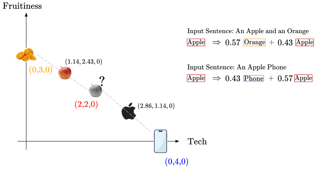
The initial embedding for the token “Apple” is the same for each possible interpretation of “Apple”, whether as a fruit or as a technology brand. By passing the tokens through the attention encoder block(s), the “Apple” token is pushed towards its context-based meaning. So, the encoder with attention layers can add contextual meaning to embeddings.

Usually, in Transformer-based architectures, there are several “encoder” blocks. Each encoder block consists of normalization layers, multi-head attention layers and a multilayer perceptron (MLP) component.

Each of these encoder blocks encodes more information into the embeddings by taking into account the context, which produces a deeper semantic representation of each token. At the end of this process, we get our optimized/improved embeddings.

To transform these information-rich embeddings into useful predictions, we need a final set of layers, which are usually called the “head”. Different heads are used for different tasks, such as classification, question-answering, Named Entity Recognition (NER), etc.

$~ \\$

The Vision Transformer works similarly, but rather than taking in word tokens, the ViT takes in image patches. Aside from that, the overall transformer architecture stays very similar for the ViT.

Next, we’ll do an overview of the ViT architecture, and make sense of the core components.

$~ \\$

2. Overview of the Vision Transformer architecture

This is the overall vision transformer architecture:

The Vision Transformer (ViT) is inspired by transformer architectures used in NLP, particularly BERT (an encoder-only transformer model).

The key idea behind ViT is to represent an image as a sequence of smaller, non-overlapping image patches, which are treated as input tokens similar to words in NLP. These patch embeddings are then processed by a transformer model, enabling the network to capture spatial relationships and patterns across the entire image.

Looking at the overall diagram, we can break the ViT into the following series of components/steps:

Transform input images into embeddings
Pass through the Transformer Encoder
Do image classification with CLS token

Next, we will run through any relevant theory for each portion, while implementing in code as we go along.

$~ \\$

3. Code-along each portion of the ViT

The changes introduced by the ViT are mostly limited to the first few processing steps, so most of the accompanying theoretical explanation will be focused on section 3.1 coming next.

$~ \\$

3.1 Transform input images into embeddings

We need to take an input image and first process it into a set of patch embeddings.

Some might ask: why not go more granular and feed in pixel values of the image directly? Well, self-attention requires comparing every input token with all other tokens (as part of learning context). If we were to process a small $32$×$32$ image at the pixel level, we would have $32^2 = 1024$ individual pixel tokens. Since self-attention has quadratic complexity (i.e., each token attends to every other token), this results in $1024^2=1,048,576$ attention computations per layer — and that’s just for a single attention layer in a multi-layer Transformer! This would be a computational nightmare.

Instead, we partition the image into patches, treating each patch as a token. These patches are then embedded into a lower-dimensional representation, significantly reducing the number of tokens while still capturing meaningful spatial information, before further processing.

Here’s a high-level overview of the steps we need to take:

Split the image into non-overlapping image patches
Embed patches into lower-dimensional embeddings via linear projection
Pre-append trainable “class” embedding to set of patch embeddings
Sum our patch embeddings with learned positional embeddings

After these steps, the patch embeddings are processed like token embeddings in a typical transformer. Let’s cover each sub-step in more detail

$~ \\$

1. Split the image into non-overlapping image patches

Splitting the image into non-overlapping image patches is a simple process, analogous to how sentences are split into tokens for NLP tasks.

Let’s assume a square image patch and define a variable, ‘patch_size’, which describes the size of our image patch, like so:

$~ \\$

2. Embed patches into lower-dimensional embeddings via linear projection

Next, we need to embed image patches into their embedded vector form. Let’s understand this mathematically.

Let’s say we’re working with $32$x$32$ input images, in RGB form. Then, our input image is a $(3, 32, 32)$ tensor, where we have $3$ channels and a $32$x$32$ shape.

Let’s say we define ‘patch_size’ to be 4, then each image patch would be a $(3, 4, 4)$ 3D tensor.

The transformer expects each token to be a flat feature vector of a fixed dimension. Let’s call the dimensionality of our desired embedding vector as ‘hidden_size’.

Since each image patch is in 3D tensor form, we need a linear projection to flatten each patch while perserving the structure, and to map the patch into a fixed-dimensional embedding vector. This operation is represented mathematically like so:

$R^{C \times P \times P} \rightarrow R^D$

Where C x P x P is the original shape of each image patch, and D is the ‘hidden_size’. This linear projection learns to extract features from the image patch, just like an embedding layer in NLP.

$~ \\$

Let’s implement the two steps above in code. To do so, we’ll define a class ‘PatchEmbeddings’ to handle splitting an input image and embedding it as vectors, based on a user defined dictionary of variables called ‘config’:

class PatchEmbeddings(nn.Module):
    """
    Converts an input image into patches, then projects patches into embedded vectors
    """

    def __init__(self, config):
        super().__init__()
        self.image_size = config["image_size"]
        self.patch_size = config["patch_size"]
        self.num_channels = config["num_channels"]
        self.hidden_size = config["hidden_size"]
        self.num_patches = (self.image_size // self.patch_size) ** 2
        self.projection = nn.Conv2d(
                self.num_channels, self.hidden_size, 
                kernel_size = self.patch_size, stride = self.patch_size
                )
    
    def forward(self, x):
        x = self.projection(x)
        x = x.flatten(2).transpose(1,2)
        return x

Notice that we use the nn.Conv2d() convolution layer to do two things at once:

Split the image into patches, by defining kernel_size and stride as patch_size
Perform a linear projection up to the number of output channels, defined by hidden_size

Let’s say our input is (B, 3, 32, 32), where we have B number of 32x32 RGB (3-channel) images, with patch_size of 4 and hidden_size of 48.

So, passing (B, 3, 32, 32) into nn.Conv2d() outputs (B, 48, 8, 8) whereby we get 8x8 = 64 patches from splitting a 32x32 image into patch of patch_size 4.

Then, passing the output (B, 48, 8, 8) into x.flatten(2).transpose(1,2), what happens is:

flatten(2) will collapse the last two dimensions (8x8) into one, so we now have (B, 48, 64)
transpose(1,2) helps us swap the axes of dimension 1 and 2, so we have (B, 64, 48). This is because transformers expect input of shape (batch_size, num_patches, embedding_dim)

Hence, each image has been transformed into a sequence of 81 embedding vectors.

$~ \\$

3. Pre-append trainable “class” embedding to set of patch embeddings

One feature introduced to transformers in the popular BERT models is the use of a [CLS] or “classification” token. The [CLS] is a special token prepended to every sentence inputted into BERT.

In BERT, the [CLS] token does not represent any word from the input, instead it serves as a global representation of the entire sequence. After passing through multiple self-attention layers, its final embedding is used for classification.

Transformers don’t have a built-in method for aggregating information. Thus, the ViT introduces a [CLS] token to:

Serve as a global representation of the entire image
Interact with all other patch embeddings via self-attention
Be used for final image classification

The [CLS] token’s embedding is learned and optimized during training.

$~ \\$

4. Sum our patch embeddings with learned positional embeddings

Transformers treat all input tokens independently at first. The Self-Attention mechanism does not inherently recognize the order or spatial position of input tokens.

What are the implications of this? Well, if we shuffle the input patches of two copies of the same image, the Vision Transformer would treat these as the same input since self-attention does not inherently track spatial positions. Then, the ViT would output the same result, which means our model has poor ability to understand images.

To preserve spatial information in ViTs, we add position embeddings to the patch embeddings before feeding them into the Transformer, like so:

$\text{Patch Embeddings + Position Embeddings} \rightarrow \text{Input to Transformer}$

There are multiple ways to introduce position embeddings in ViTs, but the standard way used in the original ViT paper is to use Learnable Position Embeddings, which have the same dimensionality as our patch embeddings.

Each patch index gets its own learnable position embedding, and during training, these embeddings are learned alongside the model.

$~ \\$

One big question I had when learning about this topic was, why do we need to use learnable position embeddings?

Earlier, we discussed the need for our model to have a spatial understanding of the image patches. Now, my question is, why do we need to use learnable position embeddings specifically?

In the simplest case, if positional encodings were not learnable, but instead hardcoded, like using the actual (x,y) coordinates of each image patch, our model might not generalize across different spatial arrangements. For example, if the positional encodings were hardcoded, our network may not be able to interpret “cat at top of image” and “cat at bottom of image” in a similar way - causing our network to obtain rigid spatial biases about the image patches.

Instead, learnable position embeddings allow the model to flexibly adapt its spatial understanding based on the data, helping it approximate or converge towards a form of translational invariance.

Furthermore, in Appendix D.4 of the original ViT paper, the authors ran an ablation study on the effects of having different positional embeddings, and found that simply having any type of learnable position embedding (whether 1D, 2D or ‘relative’) was much better than not having any positional embedding at all.

Here’s one last tidbit that might be interesting: you might notice that the additional [CLS] token we’re adding for classification is also getting a learnable positional embedding. Why?

Well, the transformer architecture does not inherently distinguish between tokens, so without a positional embedding, the [CLS] token would be treated as just another image patch, and the model wouldn’t learn that it serves a global/higher-level purpose.

In other words, having a unique learnable position embedding helps the model recognize that this token serves a special purpose. Then, through self-attention, the [CLS] token aggregates information from all patches, helping it summarize the image effectively.

$~ \\$

Let’s implement the two steps above in code. To do so, we’ll define a class ‘Embeddings’ to combine our earlier patch embeddings with the [CLS] token and position embeddings:

class Embeddings(nn.Module):
    """
    Combines original patch embeddings with [CLS] token and position embeddings
    """

    def __init__(self, config):
        super().__init__()
        self.config = config
        self.patch_embeddings = PatchEmbeddings(config)
        self.cls_token = nn.Parameter(torch.randn(1, 1, config["hidden_size"]))
        self.position_embeddings = 
            nn.Parameter(torch.randn(1, self.patch_embeddings.num_patches + 1, config["hidden_size"]))
        self.dropout = nn.Dropout(config["hidden_dropout_prob"])
    
    def forward(self, x):
        x = self.patch_embeddings(x)
        batch_size, _, _ = x.size()
        cls_tokens = self.cls_token.expand(batch_size, -1, -1)
        x = torch.cat((cls_tokens, x), dim=1)
        x = x + self.position_embeddings
        x = self.dropout(x)
        return x

Notice that we initialize self.cls_token as a single learnable token with shape (1, 1, hidden_size), which represnts (one token, batch dimension placeholder, hidden_size)
Then, we initialize the self.position_embeddings as a learnable positional embedding tensor of shape (1, num_patches + 1, hidden_size). The first 1 shows that we have a single set of positional embeddings shared across all images, then for num_patches+1, we include the [CLS] token into the total number of patches.
We also expand the single [CLS] token to match the batch_size using self.cls_token.expand(batch_size, -1, -1). The -1 tells PyTorch to keep the original size for a particular dimension.
Then, we concatenate the [CLS] token to patch embeddings along dim = 1 (the sequence length dimension)
Finally, after adding the position_embeddings, we also apply self.dropout(x) for regularization!

After this step is done, the input image is converted to a sequence of patch embeddings with positional information, ready to be fed into the transformer layer!

$~ \\$

3.2 Pass through the Transformer Encoder

In this section, we’ll build the Transformer Encoder to process our combined image patch embeddings. However, the Transformer Encoder is made up of many smaller components, as seen below:

So, we’ll focus on building the core component first, which is the Multi-Head Attention module.

$~ \\$

Multi-Head Attention Module

Multi-headed attention is used to compute the all pairwise self-attention interactions between image patches in the input image. The Multi-Head Attention Module consists of smaller attention heads, each of which computes self-attention independently over different learned feature subspaces.

So, let’s begin by implementing a single self attention head first. Recall from our other blog post that the attention head takes in a sequence of embeddings and computes the K,Q,V matrices.

class AttentionHead(nn.Module):
    """
    Single attention head
    """

    def __init__(self, hidden_size, attention_head_size, dropout, bias=True):
        super().__init__()
        self.hidden_size = hidden_size
        self.attention_head_size = attention_head_size
        self.query = nn.Linear(hidden_size, attention_head_size, bias = bias)
        self.key = nn.Linear(hidden_size, attention_head_size, bias = bias)
        self.value = nn.Linear(hidden_size, attention_head_size, bias = bias)
        self.dropout = nn.Dropout(dropout)
    
    def forward(self, x):
        query = self.query(x)
        key = self.key(x)
        value = self.value(x)
        # recall that Attention(K,Q,V) = SoftMax(QK^T/sqrt(head_size)) V
        attention_scores = torch.matmul(query, key.transpose(-1,-2)) 
        attention_scores = attention_scores / math.sqrt(self.attention_head_size)
        attention_probs = nn.functional.softmax(atention_scores, dim = -1)
        attention_probs = self.dropout(attention_probs)
        attention_output = torch.matmul(attention_probs, value)
        return(attention_output, attention_probs)

Note that attention_head_size defines the reduced dimensionality per attention head.
So, we define K,Q,V transformation matrices as a fully connected nn.Linear layer, which map the input embeddings from hidden_size to attention_head_size.

$~ \\$

In the Multi-Head Attention module, the outputs from all individual attention heads are concatenated and linearly projected to obtain the final output of the Multi-Head Attention module.

Next, to implement the Multi-Head Attention module:

class MultiHeadAttention(nn.Module):
    """
    Multi-Head Attention module
    """

    def __init__(self, config):
        super().__init__()
        self.hidden_size = config["hidden_size"]
        self.num_attention_heads = config["num_attention_heads"]
        self.attention_head_size = self.hidden_size // self.num_attention_heads
        self.all_head_size = self.attention_head_size * self.num_attention_heads
        self.kqv_bias = config["kqv_bias"]
        self.heads = nn.ModuleList([])

        for _ in range(self.num_attention_heads):
            head = AttentionHead(
                                 self.hidden_size,
                                 self.attention_head_size,
                                 config["attention_probs_dropout_prob"],
                                 self.kqv_bias
                                 )
            self.heads.append(head)
        
        self.output_projection = nn.Linear(self.all_head_size, self.hidden_size)
        self.output_dropout = nn.Dropout(config["hidden_dropout_prob"])
    
    def forward(self, x, output_attentions = False):
        attention_outputs = [head(x) for head in self.heads]
        attention_output = torch.cat([attn_output for attn_output, _ in attention_outputs], dim = -1)
        attention_output = self.output_projection(attention_output)
        attention_output = self.output_dropout(attention_output)

        if not output_attentions:
            return(attention_output, None)
        else:
            attention_probs = torch.stack([attn_probs for _, attn_probs in attention_outputs], dim = 1)
            return (attention_output, attention_probs)

Notice the seemingly strange calculation for attention_head_size and all_head_size. While it seems obvious that all_head_size is equal to hidden_size, writing the code this way provides flexibility for hidden_size and all_head_size to be different if needed, in some uncommon implementations.
Even if all_head_size == hidden_size, having the nn.Linear() layer is crucial for re-weighting and mixing the contributions of different heads.

$~ \\$

Completing the Transformer Encoder

To complete one full transformer layer, we also need to implement the MLP layer, two normalization layers and skip connections.

To implement the MLP layer, we’ll build a simple two-layer MLP with GELU activation in between:

class MLP(nn.Module):
    """
    The Multi-Layer Perceptron module
    """

    def __init__(self, config):
        super().__init__()
        self.dense_1 = nn.Linear(config["hidden_size"], config["intermediate_size"])
        self.activation = NewGELUActivation()
        self.dense_2 = nn.Linear(config["intermediate_size"], config["hidden_size"])
        self.dropout = nn.Dropout(config["hidden_dropout_prob"])
    
    def forward(self, x):
        x = self.dense_1(x)
        x = self.activation(x)
        x = self.dense_2(x)
        x = self.dropout(x)
        return x

Now that we have implemented the Multi-Headed Attention module and MLP layer, we can combine them to create the full transformer layer, along with the skip connections and layer normalization.

We’ll call this class a “Block”, since multiple transformer layers (or “blocks”) will be stacked to form the full transformer encoder.

class Block(nn.Module):
    """
    A single, full transformer layer. 
    """

    def __init__(self, config):
        super().__init__()
        self.attention = MultiHeadAttention(config)
        self.layernorm_1 = nn.LayerNorm(config["hidden_size"])
        self.mlp = MLP(config)
        self.layernorm_2 = nn.LayerNorm(config["hidden_size"])
    
    def forward(self, x, output_attentions = False):
        attention_output, attention_probs = 
            self.attention(self.layernorm_1(x), output_attentions = output_attentions)
        x = x + attention_output                    # skip connection
        mlp_output = self.mlp(self.layernorm_2(x))
        x = x + mlp_output                          # skip connection

        if not output_attentions:
            return (x, None)
        else:
            return (x, attention_probs)

Then, we’ll build the full transformer encoder, which stacks multiple transformer layers sequentially.

class Encoder(nn.Module):
    """
    Transformer Encoder module
    """

    def __init__(self, config):
        super().__init__()
        self.blocks = nn.ModuleList([])
        
        for _ in range(config["num_hidden_layers"]):
            block = Block(config)
            self.blocks.append(block)
    
    def forward(self, x, output_attentions = False):
        all_attentions = []

        for block in self.blocks:
            x, attention_probs = block(x, output_attentions = output_attentions)
            if output_attentions:
                all_attentions.append(attention_probs)
        
        if not output_attentions:
            return (x, None)
        else:
            return (x, all_attentions)

$~ \\$

3.3 Do image classification with [CLS] token

Now that the full transformer encoder is implemented, we will obtain new/optimized embeddings for the image patches and the [CLS] token!

To make these embeddings produce useful predictions, we’ll use the [CLS] token embedding as input to our classification layer.

We will implement the classification layer as a fully connected layer that takes the full [CLS] embedding of “hidden_size”, and outputs logits for each image class.

Here’s the code implementation for the full ViT classifier model:

class ViTClassifier(nn.Module):
    """
    The full ViT model for image classification
    """

    def __init__(self, config):
        super().__init__()
        self.config = config
        self.image_size = config["image_size"]
        self.hidden_size = config["hidden_size"]
        self.num_classes = config["num_classes"]
        self.embedding = Embeddings(config)
        self.encoder = Encoder(config)
        self.classifier = nn.Linear(self.hidden_size, self.num_classes)
        self.apply(self._init_weights)
    
    def forward(self, x, output_attentions = False):
        embedding_output = self.embedding(x)
        encoder_output, all_attentions = self.encoder(embedding_output, output_attentions = output_attentions)
        logits = self.classifier(encoder_output[:, 0])

        if not output_attentions:
            return (logits, None)
        else:
            return (logits, all_attentions)

    def _init_weights(self, module):
        if isinstance(module, (nn.Linear, nn.Conv2d)):
            torch.nn.init.normal_(module.weight, mean=0.0, std=self.config["initializer_range"])
            if module.bias is not None:
                torch.nn.init.zeros_(module.bias)
        elif isinstance(module, nn.LayerNorm):
            module.bias.data.zero_()
            module.weight.data.fill_(1.0)
        elif isinstance(module, Embeddings):
            module.position_embeddings.data = nn.init.trunc_normal_(
                module.position_embeddings.data.to(torch.float32),
                mean=0.0,
                std=self.config["initializer_range"],
            ).to(module.position_embeddings.dtype)

            module.cls_token.data = nn.init.trunc_normal_(
                module.cls_token.data.to(torch.float32),
                mean=0.0,
                std=self.config["initializer_range"],
            ).to(module.cls_token.dtype)

Note that _init_weights() ensures all parameters start with reasonable values, to avoid unstable training. It checks the type of layer and applies the correct model parameter initialization for all layers of the model. It uses the self.apply() function by PyTorch.

$~ \\$

4. Results

In this section, we’ll review the results from training a image classifying ViT model. The full implementation was done in a jupyter notebook, which can be found here.

Firstly, here’s a quick preview of what 32x32 images the CIFAR-10 dataset contains:

$~ \\$

I trained the model for 100 epochs, and it attained a final test accuracy of 64%.

$~ \\$

Here are two plots showing how training loss, validation loss and validation accuracy changed over the epochs:

$~ \\$

And, perhaps most interesting of all, here’s a visualization of how the model computes attention over the images. We can see that the model learned to generally focus on the key subject/class of each image, and ignore the background:

$~ \\$

To see the full code implementation, please refer to my github repo here!

$~ \\$

5. References

This project post was primarily an exercise in re-implementing and slightly modifying Trung Tin Nguyen’s excellent blog post on the ViT. I borrowed heavily from his teachings on the code implementation and theory, and I highly suggest a read through!

I also found this walkthrough of the ViT by James Briggs an excellent reference and sanity check. I also borrowed heavily from his intutive explanation of the theory, and if you already have a grasp of how Transformers work, I highly suggest this reference as your introduction to ViTs.